2歳の息子にせがまれ、きかんしゃトーマスの録画を1日2時間近く見るハメになっている。
ただ見るのもつまらないので、日本語音声と英語音声の差を楽しんでいて気が付いた。英語から日本語に直す過程で表現がだいぶマイルドになっていたり、出てくる単語や表現も偏っている。
再頻出キーワード上位に"silly(バカ)"がきっと入っているはず。
"useful engine(やくにたつきかんしゃ)"や、"fat controller(トップハムハット卿)"も、相当な回数出てきているはず。
そこで、Pythonでプログラム組んで、Webスクレイピングで全エピソードの会話を収集して集計してみた。また、Pythonを使うのは今回が初めてだったので、学習の記録を残してスキルの習得に有効な手法についても考察してみた。
台本の入手
録画した動画から音声をテキスト化して分析するのは手間がかかりすぎるので、既にテキスト化されているものがないか調べてみると、鉄道模型時代のシーズン1からシーズン12までならあった。ここから各エピソードのスクリプト(台本)にリンクが貼られている。
List of Pikachufreak's Thomas and Friends Transcripts
各リンク先ページから会話部分を抽出し、キーワードを集計してグラフ化もできるはず。
ただ、これを手作業でやるのはあまりにsillyであるので、やくにたつプログラムに処理させる。
実装手順
自然言語処理と分析、コード生成の容易さのため、Pythonで実装するのだが、自分としては今回初めての導入だった。
実行環境やライブラリの選定、構築、使い方について色々調べる中で、下記リンク先が参考になった。
今回、選定した実行環境とライブラリはこちら。
- 実行環境
- Jupyter Notebook
- Webスクレイピング
- Scrapy
- 自然言語解析
- spaCy
下記手順で処理する。
- ScrapyによるWebスクレイピング
- 各エピソードへのリンク先と、スクリプト(台本)部分の抽出のためのXPathを確認
- XPathから各リンク先と、スクリプト部分を正しく抽出できるか確認
- 一括で各リンク先からスクリプトテキストを抽出
- 順番に上から話者とセリフのテキストを取得
- json形式で保存
- jsonの読み込み
- jsonの読み込み
- 入力から解析用にデータを整形
- spaCyによる自然言語解析
- 活用形を含まない全単語を抽出し、品詞を設定
- pandasを活用して品詞ごとに集計
- 解析結果のmatplotlibによるグラフ化
- 頻出単語を水平棒グラフで確認
- 単語の出現順位と出現回数を散布図で確認
ScrapyによるWebスクレイピング
Scrapyを使ってList of Pikachufreak's Thomas and Friends Transcripts から各要素を抽出する。
- XPathの抽出
- リンク先の確認
- 抽出するテキストの確認
- 各リンク先よりスクリプトを抽出
- json形式で保存
基本的に、チュートリアルに沿って改変すればOK Scrapy Tutorial
URLを開き、ページ中の特定の箇所からテキストを抜き出すスパイダーを作り、クロールさせる。
各リンク先と、スクリプト(台本)部分の抽出のためのXPathを確認
まずは、ページの中のどこに抜き出したい部分があるのか調べる必要がある。XPathを使うと、cssセレクタを使うよりも高度な選択ができる。
チュートリアル:XPath: a brief intro
Chrome拡張機能のSelector gadgetや、開発者ツールを利用するとよい。
- トップページから各ページへのリンク
//ol//a/@href
- 各ページのテキスト部分
-
//*[(@id = "mw-content-text")]//ul//li/text()全部 -
//*[(@id = "mw-content-text")]//ul[2]//li/text()登場人物 -
//*[(@id = "mw-content-text")]//ul[3]//li/text()スクリプト本体
-
XPathから各リンク先と、スクリプト部分を正しく抽出できるか確認
スクリプトのある各ページへのリンクを、調べたXPathから正しく取得できるか確認する。
チュートリアル:Extracting data
対話的にscrapy shellで確認する。
scrapy shell
"http://scratchpad.wikia.com/wiki/List_of_Pikachufreak's_Thomas_and_Friends_Transcripts"
全部確認する。
In [15]: response.xpath('//ol//a/@href').extract()
Out[15]:
['/wiki/Thomas_Gets_Tricked_Transcript',
 '/wiki/Edward_Helps_Out_Transcript',
 (省略)
 '/wiki/Come_Out_Henry_Transcript',
 '/wiki/Best_Friends_Transcript']
各リンク先からスクリプトテキストを抽出できるか確認
スクリプトのある各ページのテキストを、調べたXPathから正しく取得できるか確認する。
同様に、対話的にscrapy shellで確認する。
scrapy shell "http://scratchpad.wikia.com/wiki/Thomas_Gets_Tricked_Transcript"
試しに、登場人物に該当する部分を取得する。
In [16]: response.xpath('//*[(@id = "mw-content-text")]//ul[2]//li/text()').extr
    ...: act()
Out[16]:
[' Thomas\n',
 ' Gordon\n',
 ' Henry (',
 ')\n',
 ' James (',
 ')\n',
 ' Clarabel (',
 ')\n',
 ' Sir Topham Hatt (',
 ')\n',
 ' Stephen Hatt (',
 ')\n',
 ' Jeremiah Jobling (',
')\n']
<i></i>タグの部分を含めるとき、|でつなぐ。
In [18]: response.xpath('//*[(@id = "mw-content-text")]//ul[2]//li/text()|//ul[2
    ...: ]//i/text()').extract()
Out[18]:
[' Thomas\n',
 ' Gordon\n',
 ' Henry (',
 'cameo',
 ')\n',
 ' James (',
 'cameo',
 ')\n',
 ' Clarabel (',
 'cameo',
 ')\n',
 ' Sir Topham Hatt (',
 'cameo',
 ')\n',
 ' Stephen Hatt (',
 'cameo',
 ')\n',
 ' Jeremiah Jobling (',
 'cameo',
 ')\n']
一括で各リンク先よりスクリプトを抽出
クロールさせるスパイダーを作成する。
チュートリアル:More examples and patterns
import scrapy


class TranscriptSpider(scrapy.Spider):
    name = 'transcript'

    start_urls = ["http://scratchpad.wikia.com/wiki/List_of_Pikachufreak's_Thomas_and_Friends_Transcripts"]

    def parse(self, response):
        # follow links to each episode's pages
        for href in response.xpath('//ol//a/@href'):
            episode_title = response.xpath('//ol//a/text()').extract_first()
            yield response.follow(href, self.parse_transcript)

    def parse_transcript(self, response):
        def extract_with_xpath(query):
            return response.xpath(query).extract()

        yield {
            'transcript': extract_with_xpath('//*[(@id = "mw-content-text")]//ul[3]//li/text()'),
        }
シーズン名、エピソードタイトルなしだが、これで全エピソードの会話部分を抽出できる。
scrapy crawl transcript
json形式で保存
Feed exportを使い、-oオプションでファイル名を指定する。
チュートリアル:Storing the scraped data
scrapy crawl transcript -o transcript.json
jsonの読み込み
Scrapyからtranscript.jsonを出力できた。ファイルを読み込み、必要な部分を自然言語解析できるようにする。
まずは、先頭を確認してみる。[リスト(各ページごと){辞書(今回はkey1つのみ)[リスト(ページ内で該当する部分全て)]}]の順で入れ子になっている。
head -n 3 transcript.json
[
{"transcript": [" Ringo Starr: Thomas is a tank engine who lives at the big station on the Island of Sodor. (省略)" Ringo Starr: Thomas thought to himself. And he puffed slowly home.\n"]},
{"transcript": [" ", ": One day, Edward was in the shed where he live with the other engines. (省略) ": I'll get out my paint tomorrow, and give you your beautiful coat of blue with red stripes, then you'll be the smartest engine in the shed.\n"]},
jsonファイルを読み込み、最初のページの1段落分だけ確認する。
import json

f = open('transcript.json', 'r')
json_dict = json.load(f)
print('number of episodes: {}'.format(len(json_dict)))
print('number of conversation: {}'.format(len(json_dict[0]['transcript'])))
print('transcript: {}'.format(json_dict[0]['transcript'][0]))
number of episodes: 308
number of conversation: 35
transcript:  Ringo Starr: Thomas is a tank engine who lives at the big station on the Island of Sodor. He's a cheeky little engine with 6 small wheels, a short stumpy funnel, a short stumpy boiler and a short stumpy dome. He's a fussy little engine too. Always pulling coaches about ready for the big engines can take on long journeys. And when trains come in, he pulls the empty coaches away so that the big engines can go on rest. Thomas thinks no engine works has hard as he does. He loves playing tricks on them, including Gordon the biggest and proudest engine of all. Thomas likes to tease Gordon with his whistle.
先頭の発話者の名前を除外してカウントするため、":"以降の文字列を切り取る。
w = json_dict[0]['transcript'][0]
if not w.find(':') == -1:
    begin = w.find(':') + 2
    w = w[begin:]
print(w)
Thomas is a tank engine who lives at the big station on the Island of Sodor. He's a cheeky little engine with 6 small wheels, a short stumpy funnel, a short stumpy boiler and a short stumpy dome. He's a fussy little engine too. Always pulling coaches about ready for the big engines can take on long journeys. And when trains come in, he pulls the empty coaches away so that the big engines can go on rest. Thomas thinks no engine works has hard as he does. He loves playing tricks on them, including Gordon the biggest and proudest engine of all. Thomas likes to tease Gordon with his whistle.
spaCyによる自然言語解析
JSONファイルから処理したい文字列を読み取れた。各文字列をspaCyで自然言語解析し、結果を確認する。
- 各文字列から活用形を含まない単語を抽出し、品詞を設定
- dataframeにエピソード通し番号/単語/品詞をセットし、csvファイルをエクスポート
- csvファイルを開き、名詞(NOUN)/形容詞(ADJ)/動詞(VERB)ごとの単語出現回数を数える
spaCyのインストール
GET STARTEDに従い、本体をインストールする。
pip3 install -U spacy
英語モデルをダウンロードする。
python -m spacy download en
エラーが出て失敗することもある。
<urlopen error [SSL: CERTIFICATE_VERIFY_FAILED] certificate verify failed (_ssl.c:833)>
エラーが出たときはこちらを参照して、ルート証明書の設定をする。
macOS用公式インストーラーのPython 3.6でCERTIFICATE_VERIFY_FAILEDとなる問題
活用形を含まない全単語を抽出し、dataframeにしてcsvエクスポート
Part-of-speech taggingを参考に、コードを書く。まずは、最初のページの1段落分だけdataframeをセットして確認してみる。
DataFrameにセットするやり方はこちらを参考にした。
from pandas import DataFrame, read_csv
import matplotlib.pyplot as plt
import pandas as pd
import spacy

nlp = spacy.load('en_core_web_sm')

index_e = []

tokens = []
lemma = []
pos = []
df = pd.DataFrame()

i = 0
w = json_dict[i]['transcript'][0]
if not w.find(':') == -1:
    begin = w.find(':') + 2
    w = w[begin:]
doc = nlp(w)

for token in doc:
    index_e.append(i)
    tokens.append(token.text)
    lemma.append(token.lemma_)
    pos.append(token.pos_)

df['index_e'] = index_e
df['tokens'] = tokens
df['lemma'] = lemma
df['pos'] = pos
df
| index_e | tokens | lemma | pos | |
|---|---|---|---|---|
| 0 | 0 | Thomas | thomas | PROPN |
| 1 | 0 | is | be | VERB |
| 2 | 0 | a | a | DET |
| 3 | 0 | tank | tank | NOUN |
| 4 | 0 | engine | engine | NOUN |
| 5 | 0 | who | who | NOUN |
| 6 | 0 | lives | live | VERB |
| 7 | 0 | at | at | ADP |
| 8 | 0 | the | the | DET |
| 9 | 0 | big | big | ADJ |
| 10 | 0 | station | station | NOUN |
| 11 | 0 | on | on | ADP |
| 12 | 0 | the | the | DET |
| 13 | 0 | Island | island | PROPN |
| 14 | 0 | of | of | ADP |
| 15 | 0 | Sodor | sodor | PROPN |
| 16 | 0 | . | . | PUNCT |
| 17 | 0 | He | -PRON- | PRON |
| 18 | 0 | 's | be | VERB |
| 19 | 0 | a | a | DET |
| 20 | 0 | cheeky | cheeky | ADJ |
| 21 | 0 | little | little | ADJ |
| 22 | 0 | engine | engine | NOUN |
| 23 | 0 | with | with | ADP |
| 24 | 0 | 6 | 6 | NUM |
| 25 | 0 | small | small | ADJ |
| 26 | 0 | wheels | wheel | NOUN |
| 27 | 0 | , | , | PUNCT |
| 28 | 0 | a | a | DET |
| 29 | 0 | short | short | ADJ |
| ... | ... | ... | ... | ... |
| 96 | 0 | he | -PRON- | PRON |
| 97 | 0 | does | do | VERB |
| 98 | 0 | . | . | PUNCT |
| 99 | 0 | He | -PRON- | PRON |
| 100 | 0 | loves | love | VERB |
| 101 | 0 | playing | play | VERB |
| 102 | 0 | tricks | trick | NOUN |
| 103 | 0 | on | on | ADP |
| 104 | 0 | them | -PRON- | PRON |
| 105 | 0 | , | , | PUNCT |
| 106 | 0 | including | include | VERB |
| 107 | 0 | Gordon | gordon | PROPN |
| 108 | 0 | the | the | DET |
| 109 | 0 | biggest | big | ADJ |
| 110 | 0 | and | and | CCONJ |
| 111 | 0 | proudest | proudest | ADJ |
| 112 | 0 | engine | engine | NOUN |
| 113 | 0 | of | of | ADP |
| 114 | 0 | all | all | DET |
| 115 | 0 | . | . | PUNCT |
| 116 | 0 | Thomas | thomas | PROPN |
| 117 | 0 | likes | like | VERB |
| 118 | 0 | to | to | PART |
| 119 | 0 | tease | tease | VERB |
| 120 | 0 | Gordon | gordon | PROPN |
| 121 | 0 | with | with | ADP |
| 122 | 0 | his | -PRON- | ADJ |
| 123 | 0 | whistle | whistle | NOUN |
| 124 | 0 | . | . | PUNCT |
| 125 | 0 | \n | \n | SPACE |
126 rows × 4 columns
pandasのdataframeを使えば、行数が多くても最初と最後の30行だけ確認できて便利。正しく抽出できていそうなので、全シーズン、全エピソードで処理する。
index_e = []
tokens = []
lemma = []
pos = []
df = pd.DataFrame()

for i,v in enumerate(json_dict):
    print('i: {}'.format(i))
    for j,w in enumerate(v['transcript']):
        if not w.find(':') == -1 :
            begin = w.find(':') + 2
            w = w[begin:]
        print('transcript: {}'.format(w[:60]))
        doc = nlp(w)
        for token in doc:
            index_e.append(i)
            tokens.append(token.text)
            lemma.append(token.lemma_)
            pos.append(token.pos_)

df['index_e'] = index_e
df['tokens'] = tokens
df['lemma'] = lemma
df['pos'] = pos
df
i: 0
transcript: Thomas is a tank engine who lives at the big station on the
transcript: Wake up, lazybones. Why don't you work hard like me?

(省略)

i: 1
transcript:
transcript: One day, Edward was in the shed where he live with the other

(省略)

i: 307
transcript:
transcript: It was a beautiful morning on the Island of Sodor. Thomas th
transcript:
transcript: Hello, Thomas

(省略)

transcript:
transcript: And I'm sorry I teased you. Your green paint look splendid a
| index_e | tokens | lemma | pos | |
|---|---|---|---|---|
| 0 | 0 | Thomas | thomas | PROPN |
| 1 | 0 | is | be | VERB |
| 2 | 0 | a | a | DET |
| 3 | 0 | tank | tank | NOUN |
| (省略) | ||||
| ... | ... | ... | ... | ... |
| (省略) | ||||
| 154892 | 307 | coal | coal | NOUN |
| 154893 | 307 | . | . | PUNCT |
| 154894 | 307 | \n | \n | SPACE |
154895 rows × 4 columns
句読点含めて15万語ほど、正しく処理できていそう。csvファイルで保存しておく。
df.to_csv('tokens.csv',index=False)
品詞の集計
出力したcsvを読み込む。
Location = 'tokens.csv'
df = pd.read_csv(Location)
df
| index_e | tokens | lemma | pos | |
|---|---|---|---|---|
| 0 | 0 | Thomas | thomas | PROPN |
| 1 | 0 | is | be | VERB |
| 2 | 0 | a | a | DET |
| 3 | 0 | tank | tank | NOUN |
| (省略) | ||||
| ... | ... | ... | ... | ... |
| (省略) | ||||
| 154890 | 307 | careful | careful | ADJ |
| 154891 | 307 | of | of | ADP |
| 154892 | 307 | coal | coal | NOUN |
| 154893 | 307 | . | . | PUNCT |
| 154894 | 307 | \n | \n | SPACE |
154895 rows × 4 columns
正しくcsvを読み込んでdataframeをセットできた。
品詞ごとに単語数をカウント
全単語を集計する。
df['lemma'].value_counts()
.              15785
-PRON-         12871
\n             11798
be              6354
the             6101
,               4218
to              3024
and             2995
                2130
a               1880
thomas          1586
not             1497
!               1461
have            1380
do              1197
but             1052
of              1039
sir              974
engine           963
percy            913
will             865
?                797
on               789
that             780
say              748
at               679
in               679
hatt             673
for              669
topham           663
               ...
type               1
whoos              1
farth              1
takeaway           1
maintenance        1
non                1
hog                1
submarine          1
lovingly           1
innocently         1
coughs             1
got                1
sundown            1
yawned             1
mishap             1
sharp              1
inquired           1
indignantly        1
makeup             1
hiccup             1
boxy               1
sheet              1
painful            1
crumbling          1
sobbed             1
sulky              1
center             1
mummy              1
preserve           1
serge              1
Name: lemma, Length: 3495, dtype: int64
品詞ごとの単語総数を集計する。
df.groupby(['pos'])['lemma'].count()
pos
ADJ       9154
ADP       8210
ADV      10500
CCONJ     4118
DET      10013
INTJ       996
NOUN     18054
NUM        381
PART      3712
PRON     10972
PROPN    13215
PUNCT    23323
SPACE    14198
VERB     28044
X            5
Name: lemma, dtype: int64
品詞それぞれの単語ごとの総数を集計する。
df.groupby(['pos'])['lemma'].value_counts()
pos   lemma
ADJ   -PRON-       1917
      good          314
      all           187
      old           181
      new           176
      other         148
      next          146
      big           138
      special       124
      little        121
      important     120
      sorry         116
      happy         110
      late          110
      useful        109
      silly         100
      last           98
      more           98
      right          94
      bad            82
      long           77
      sure           74
      ready          73
      busy           71
      heavy          71
      pleased        67
      red            60
      wrong          58
      worried        57
      that           56
                   ...
VERB  tuck            1
      tune            1
      twa             1
      twink           1
      unloaded        1
      utter           1
      vanish          1
      venture         1
      vow             1
      waddle          1
      weaken          1
      wedge           1
      wheel           1
      whees           1
      whimper         1
      whirl           1
      whiz            1
      whoos           1
      widen           1
      winch           1
      windbreak       1
      wipe            1
      wire            1
      wreck           1
      yard            1
      zoom            1
X     ho              2
      >               1
      bon             1
      osh             1
Name: lemma, Length: 4442, dtype: int64
特定の品詞のみの単語ごとの総数を取り出す。まずは形容詞。
df[df['pos'] == 'ADJ']['lemma'].value_counts()
-PRON-           1917
good              314
all               187
old               181
new               176
other             148
next              146
big               138
special           124
little            121
important         120
sorry             116
happy             110
late              110
useful            109
silly             100
more               98
last               98
right              94
bad                82
long               77
sure               74
ready              73
busy               71
heavy              71
pleased            67
red                60
wrong              58
worried            57
that               56
                 ...
chirpy              1
tremendous          1
fruitless           1
damaged             1
satisfied           1
decent              1
medical             1
buttered            1
unaware             1
bleak               1
squat               1
piled               1
outside             1
sagacious           1
alright             1
impossible          1
tiresome            1
nuisance            1
revolutionary       1
springtime          1
guarateed           1
shameful            1
loneliness          1
odd                 1
tasty               1
pleasant            1
aah                 1
snap                1
embarrassing        1
shunted             1
Name: lemma, Length: 624, dtype: int64
次は、名詞の単語ごと総数をカウントする。
df[df['pos'] == 'NOUN']['lemma'].value_counts()
engine         915
car            609
driver         479
what           397
line           312
time           300
freight        293
day            257
station        254
sir            228
train          226
coach          180
percy          174
work           173
way            160
passenger      152
child          142
morning        142
everyone       137
coal           133
yard           117
trouble        109
shed           107
night          106
job            105
fireman        104
cross          103
who            103
track          103
wheel           98
              ...
team             1
runaway          1
tongue           1
mister           1
bout             1
dance            1
character        1
singer           1
crackpot         1
sunlight         1
escape           1
bouncy           1
butler           1
banana           1
snowball         1
mark             1
goblin           1
fury             1
shortage         1
can              1
whip             1
lighthouse       1
wail             1
grove            1
lighting         1
destruction      1
trial            1
example          1
clickity         1
gown             1
Name: lemma, Length: 1626, dtype: int64
続いて、動詞の単語ごと総数をカウントする。
df[df['pos'] == 'VERB']['lemma'].value_counts()
be           6354
have         1380
do           1197
will          865
say           748
go            626
see           490
can           464
come          451
take          394
get           347
look          325
puff          325
could         319
make          310
know          308
think         303
would         278
feel          268
stop          266
pull          252
help          239
want          230
tell          222
wait          220
arrive        219
must          217
work          200
call          187
hear          169
             ...
shove           1
side            1
host            1
purpose         1
chip            1
gain            1
barge           1
firm            1
gloat           1
cricket         1
swap            1
butch           1
meetsthe        1
agreed          1
teeter          1
power           1
overjoy         1
dismay          1
squelch         1
slunk           1
sell            1
funnel          1
gallivant       1
bunker          1
plummet         1
outlast         1
coast           1
trickle         1
saw             1
serge           1
Name: lemma, Length: 1010, dtype: int64
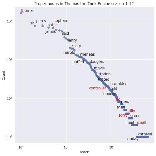
同様に、固有名詞の単語ごと総数をカウントする。
df[df['pos'] == 'PROPN']['lemma'].value_counts()
thomas         1586
sir             746
percy           738
hatt            673
topham          663
james           587
gordon          569
said            534
toby            379
henry           350
edward          318
duncan          202
rusty           191
skarloey        191
duck            177
harold          130
sodor           127
oliver          127
bertie          119
rheneas         116
sam             115
peter           114
bill            107
diesel          106
puffed           97
ben              95
island           94
cried            88
clarabel         82
annie            81
               ...
careful           1
wearily           1
oh                1
jeered            1
comfy             1
choked            1
hovered           1
whirled           1
mmmm              1
hault             1
birdbrain         1
cander            1
announced         1
crossing          1
grr               1
packard           1
puff              1
troublesome       1
buzzed            1
fusspot           1
chirped           1
dirty             1
windmill          1
factory           1
adventure         1
muddle            1
home              1
ease'll           1
wait'll           1
gruffed           1
Name: lemma, Length: 615, dtype: int64
最後に、特定の単語の順位と出現回数を品詞別に調べる。全品詞と形容詞、名詞で分ける。groupbyから得たSeries型にindex名を[[('pos','lemma')]]のように指定してやると、値である出現回数を取り出せる。しかし、index名からindex番号である順位を取り出すやり方が分からなかった。そこで、次のようなやり方をとる。
- 新しくdataframeを作り、順位はindex番号+1とする
-
text列はindex名とする -
count列は値とする - 特定の単語について、表示用のdataframeにコピーして表示する
もっといいやり方はきっとあるはずだが、これでやっつける。
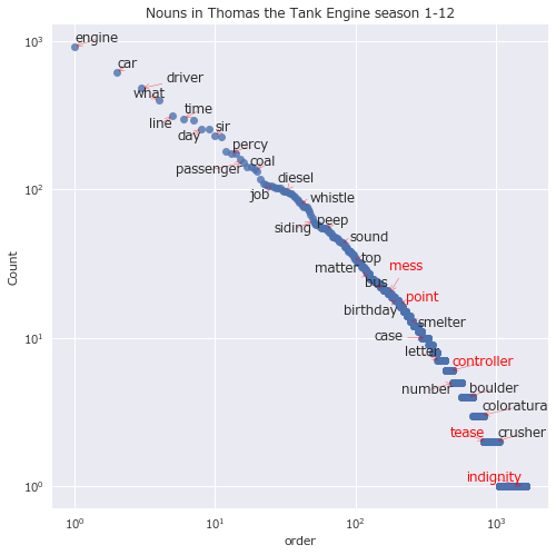
interest_word = ["silly","useful","engine","sorry","tease","indignity","mess","fat","controller","small","point"]

df_ord = {}
df_ord['all'] = pd.DataFrame() # 新しくdataframeを作る
df_ord['all']['text'] = df['lemma'].value_counts().index # `text`列はindex名とする
df_ord['all']['count'] = df['lemma'].value_counts().values # `count`列は値とする
df_ord['ADJ'] = pd.DataFrame()
df_ord['ADJ']['text'] = df[df['pos'] == 'ADJ']['lemma'].value_counts().index
df_ord['ADJ']['count'] = df[df['pos'] == 'ADJ']['lemma'].value_counts().values
df_ord['NOUN'] = pd.DataFrame()
df_ord['NOUN']['text'] = df[df['pos'] == 'NOUN']['lemma'].value_counts().index
df_ord['NOUN']['count'] = df[df['pos'] == 'NOUN']['lemma'].value_counts().values

print('Order in all {} words'.format(df['lemma'].value_counts().size))
df_print = pd.DataFrame()
for word in interest_word: # 特定の単語について、表示用のdataframeにコピーして表示
    df_print = pd.concat([df_print, df_ord['all'][df_ord['all']['text'] == word]])
print(df_print.sort_values(by="count", ascending=False),'\n')

print('Order in adjective {} words'.format(df[df['pos'] == 'ADJ']['lemma'].value_counts().size))
df_print = pd.DataFrame()
for word in interest_word:
    df_print = pd.concat([df_print, df_ord['ADJ'][df_ord['ADJ']['text'] == word]])
print(df_print.sort_values(by="count", ascending=False),'\n')

print('Order in noun {} words'.format(df[df['pos'] == 'NOUN']['lemma'].value_counts().size))
df_print = pd.DataFrame()
for word in interest_word:
    df_print = pd.concat([df_print, df_ord['NOUN'][df_ord['NOUN']['text'] == word]])
print(df_print.sort_values(by="count", ascending=False),'\n')
Order in all 3495 words
            text  count
18        engine    963
136        sorry    143
173       useful    109
183        silly    104
303        tease     54
475        small     31
511   controller     27
576        point     23
607         mess     21
959          fat     10
3194   indignity      1

Order in adjective 624 words
       text  count
11    sorry    116
14   useful    109
15    silly    100
64    small     29
569     fat      1

Order in noun 1626 words
            text  count
0         engine    915
177         mess     20
201        point     17
467   controller      6
1039       tease      2
1289   indignity      1
きかんしゃトーマスでは、やはり相当な回数'silly(バカ)'とか'useful(やくにたつ)'と言っており、それ以上に'sorry'と謝ってばかりいた。
案外、"fat controller"とは言ってなさそうだ。どうやら、UK版とUS版でセリフが違うらしい。
解析結果のmatplotlibによるグラフ化とseabornによるスタイル変更
気になるキーワードの出現回数や順位は分かったものの、まだ全体の中での位置付けが分かりづらいので、グラフ化して確認する。頻出単語は水平棒グラフで確認し、単語出現順位と出現回数は散布図にラベルを付けて確認する。
- PythonでPandasのPlot機能を使えばデータ加工からグラフ作成までマジでシームレス
- matplotlibで棒グラフを作る
- seabornで簡単に見栄えを良くする
- グラフの大きさを調整する
- 軸を反転させる
- 軸タイトルを付ける
まずは、PandasのPlot機能で簡単に確認する。
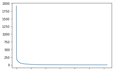
%matplotlib inline

df[df['pos'] == 'ADJ']['lemma'].value_counts().plot()
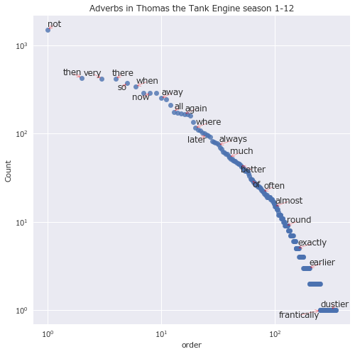
ラベルを付けて数値を確認したい。全体の中の一部分、先頭20個分を水平棒グラフにする。
df[df['pos'] == 'ADJ']['lemma'].value_counts().head(20).plot.barh()

PandasのPlot機能で簡単に確認できたものの、色がバラバラになるのは避けたいし、もう少し見やすくしたい。グラフの体裁を整える。
- 使えるフォントを調べる
- seabornの適用
- matplotlibでグラフ作成
- 大きさを調整
- ラベルを付ける
- 逆順にして水平棒グラフ作成
- 出現順位と出現回数で散布図作成
使えるフォントを調べる。
import matplotlib.font_manager
print([f.name for f in matplotlib.font_manager.fontManager.ttflist])
['STIXSizeThreeSym', 'STIXSizeTwoSym', 'cmr10', 'STIXNonUnicode', 'DejaVu Sans Mono', 'DejaVu Serif', (省略), 'Meiryo']
seabornスタイルを適用する。
- グリッドはdarkgrid
- フォントはMeiryo
import seaborn as sns
sns.set(style="darkgrid", font='Meiryo')
描画用にdataframeを作成し、はじめの21個だけ確認する。
df_s = df[df['pos'] == 'ADJ']['lemma'].value_counts()
df_ex = pd.DataFrame()
df_ex['text'] = df_s.index
df_ex['count'] = df_s.values
df_ex = df_ex[:20]
df_ex
| text | count | |
|---|---|---|
| 0 | -PRON- | 1917 |
| 1 | good | 314 |
| 2 | all | 187 |
| 3 | old | 181 |
| 4 | new | 176 |
| 5 | other | 148 |
| 6 | next | 146 |
| 7 | big | 138 |
| 8 | special | 124 |
| 9 | little | 121 |
| 10 | important | 120 |
| 11 | sorry | 116 |
| 12 | happy | 110 |
| 13 | late | 110 |
| 14 | useful | 109 |
| 15 | silly | 100 |
| 16 | more | 98 |
| 17 | last | 98 |
| 18 | right | 94 |
| 19 | bad | 82 |
Matplotlibで水平棒グラフを作成する。
fig, ax = plt.subplots(figsize=(8, 8)) #大きさを指定してサブプロット作成
ax.barh(df_ex['text'], df_ex['count']) #X軸とY軸を指定して、水平棒グラフ作成。X軸とY軸が入れ替わる。
plt.xlabel('Count') #ラベルを付ける
plt.title("Adjectives in Thomas the Tank Engine season 1 first paragraph")
ax.invert_yaxis() #Y軸(df_ex.index)を反転させる
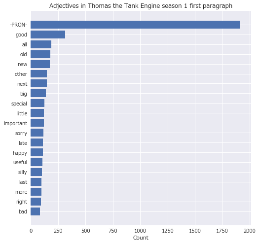
水平棒グラフで頻出単語の出現回数を確認できた。単語の出現順位と回数の関係は、散布図にラベルを付けて確認する。ここで、次のようにする。
- adjustTextで文字が重ならないようにする
- 対数間隔でラベルを間引く
- 対数軸でプロットする
文字が重ならないようにするためには、adjustTextライブラリがとても役に立つ。ライブラリをインポート。
from adjustText import adjust_text
50個おきにラベルを付けて全体を散布図でプロットする。
texts = []
df_s = df[df['pos'] == 'ADJ']['lemma'].value_counts()
df_ex = pd.DataFrame()
df_ex['text'] = df_s.index
df_ex['count'] = df_s.values
df_ex = df_ex[1:]

fig, ax = plt.subplots(figsize=(8,8))
ax.plot(df_ex.index, df_ex['count'],'o',alpha=0.8)
plt.xlabel('Count')
plt.ylabel('order')
plt.title("Adjectives in Thomas the Tank Engine season 1-12")

for k, v in df_ex.iterrows():
    if v[0] in interest_word:
        texts.append(plt.text(k,v[1],v[0],color='red'))
    else:
        if k%50 == 1:
            texts.append(plt.text(k,v[1],v[0]))
adjust_text(texts, arrowprops=dict(arrowstyle='-', color='red'))
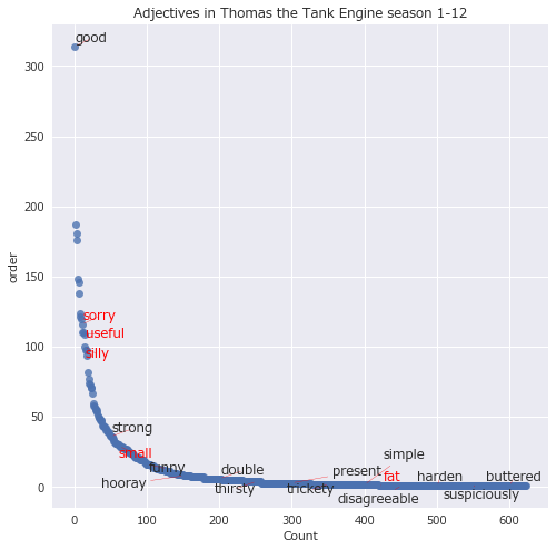
全体を見てみると、出現回数の多い単語は少なく、出現回数の少ない単語は多い。出現回数の多いものほどたくさんラベルが付くように、対数間隔でラベルを間引く。
import numpy as np

t1 = np.logspace(0,3,31)
print(t1)
t10 = np.round(t1)
print(t10)
[   1.            1.25892541    1.58489319    1.99526231    2.51188643
    3.16227766    3.98107171    5.01187234    6.30957344    7.94328235
   10.           12.58925412   15.84893192   19.95262315   25.11886432
   31.6227766    39.81071706   50.11872336   63.09573445   79.43282347
  100.          125.89254118  158.48931925  199.5262315   251.18864315
  316.22776602  398.10717055  501.18723363  630.95734448  794.32823472
 1000.        ]
[   1.    1.    2.    2.    3.    3.    4.    5.    6.    8.   10.   13.
   16.   20.   25.   32.   40.   50.   63.   79.  100.  126.  158.  200.
  251.  316.  398.  501.  631.  794. 1000.]
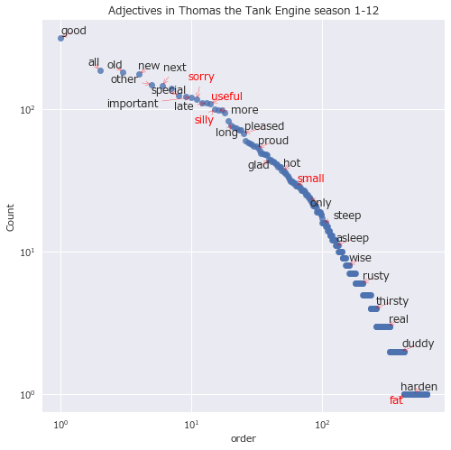
対数軸で全体をプロットする。まずは形容詞。
texts = []
df_s = df[df['pos'] == 'ADJ']['lemma'].value_counts()
df_ex = pd.DataFrame()
df_ex['text'] = df_s.index
df_ex['count'] = df_s.values
df_ex = df_ex[1:]

fig, ax = plt.subplots(figsize=(8,8))
ax.plot(df_ex.index, df_ex['count'],'o',alpha=0.8)
plt.xlabel('order')
plt.ylabel('Count')
plt.title("Adjectives in Thomas the Tank Engine season 1-12")
ax.set_xscale('log')
ax.set_yscale('log')

for k, v in df_ex.iterrows():
    if v[0] in interest_word:
        texts.append(plt.text(k,v[1],v[0], color='red'))
    else:
        if k in t10:
            texts.append(plt.text(k,v[1],v[0]))
adjust_text(texts, arrowprops=dict(arrowstyle='->', color='red'))
同様に名詞をプロット。
texts = []
df_s = df[df['pos'] == 'NOUN']['lemma'].value_counts()
# 以下同様
動詞をプロット。
texts = []
df_s = df[df['pos'] == 'VERB']['lemma'].value_counts()
# 以下同様
副詞をプロット。
texts = []
df_s = df[df['pos'] == 'ADV']['lemma'].value_counts()
# 以下同様
固有名詞をプロット。
texts = []
df_s = df[df['pos'] == 'PROPN']['lemma'].value_counts()
# 以下同様
全部プロット。
texts = []
df_s = df['lemma'].value_counts()
# 以下同様
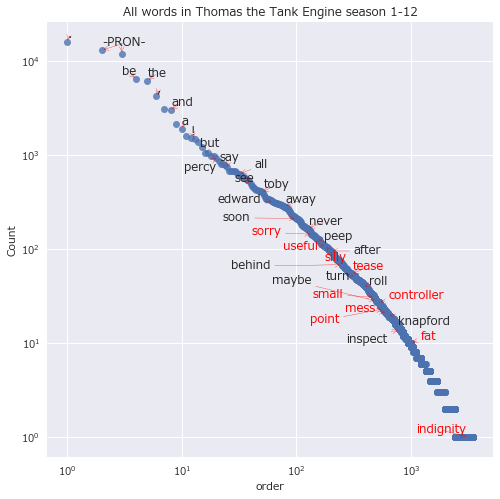
どの品詞にしても、出現順位のおおよそ-1乗に比例して出現回数が少なくなっていそうだ。
2018/7/11追記:
直近1年のQiita記事分析で分かった7つの「驚愕」へのtakotakotさんのコメントを見て、ジップの法則を知った。
ジップの法則(ジップのほうそく、Zipf's law)あるいはジフの法則とは、出現頻度が k 番目に大きい要素が全体に占める割合が 1/k に比例するという経験則である。
今回の結果はジップの法則の由来そのもののようだ。
元来は、アメリカの言語学者ジョージ・キングズリー・ジップが英語の単語の出現頻度とその順位に関して発見した言語学の法則である。
まとめ
- ScrapyでWebスクレイピングして、鉄道模型時代のきかんしゃトーマスの全12シーズン分のスクリプトをjsonファイルに書き出せた
- spaCyで自然言語解析して、pandasのdataframeを活用してほぼ品詞別に頻出キーワードを整理できた
- "silly(バカ)":形容詞 16/624位 100回
- "useful(やくにたつ)":形容詞 15/624位 109回
- "engine(きかんしゃ)":名詞 1/1626位 915回
- "fat(デブ)":形容詞 570/1176位 1回
- "controller(司令官)":名詞 467/1626位 6回
- 頻出キーワードを整理した結果、予想通りだった部分と意外な部分が分かった
- 予想通り、"silly"や"useful"は頻出キーワード上位に入った
- どうやらUS版は本家UK版とは違って教育的配慮がなされているのか、トップハム・ハット卿は"The Fat Controller(デブ司令官)"と呼ばれていなかった
- 結果をMatplotlibでグラフ化してみることで、全体の中での位置付けや特徴を把握できた
- 対数グラフにしてみると、出現順位のおおよそ-1乗に比例して出現回数が少なくなっていそうで、ジップの法則を確認した
- ラベルどうしが重ならないよう、ラベルを重ね書きすることで、着目した単語の位置付けが分かりやすくなった
- スキルの取得に有効な手法を試すことができた
- 使えそうなチュートリアルを試し、チュートリアルのコードを改変して目的のコードを作る
- チュートリアルやリファレンスは全部やろうとすると際限ないので、全部やらない
- 完成度を高めようと情報を探し始めるとキリがなく、いつまでたっても終わらないので、適当なところで手を置いて未着手の部分をやる
頻出キーワード分析やるなら、TOEICや英検、センター模試など英語試験を題材にした方がよっぽど役に立ってよかった気もするけど、後悔はしていない。20年近く英語を勉強したり使い続けていたものの、初めて見るような単語が上位に入っていた。"coach(客車)"や"freight(貨車)"とか。驚くべきことに、自分の英語力は子供向け番組の語彙レベルに達していなかった。