日本語コメントつきTensorFlow MNIST Begginer/Expertのコード

TensorFlowのチュートリアルMNISTのコードに日本語コメントが書かれたものをたくさんの方が書かれていて学習時にとても役に立ったので自分なりのものもまとめました。
(間違いなど見つけた方あればご指摘いただけるとうれしいですmm)

MNIST For ML Beginners

# coding: utf-8

# データの読み込み
from tensorflow.examples.tutorials.mnist import input_data
mnist = input_data.read_data_sets("MNIST_data/", one_hot=True)

# tensorflow を tf として読み込み
import tensorflow as tf

# y = softmax(x*W + b)を定義していく
## x を[?, 784]のテンソルとして定義(Noneは何個入るかわからないという意味)
x = tf.placeholder(tf.float32, [None, 784])

## W を[784, 10]のテンソルとして定義。784個の各ピクセル×0〜9までの各数字分。
W = tf.Variable(tf.zeros([784, 10]))

## b を[10](全て0で初期化)のテンソルとして定義。0〜9までの各値のバイアス
b = tf.Variable(tf.zeros([10]))

## 定義した各変数を式に当てはめていく
## matmulは行列の積算を行う関数
y = tf.nn.softmax(tf.matmul(x, W) + b)

# y_(ラベル)を [?, 10]のテンソルとして定義
y_ = tf.placeholder(tf.float32, [None, 10])

# cross_entropyを定義
cross_entropy = tf.reduce_mean(-tf.reduce_sum(y_  * tf.log(y), reduction_indices=[1]))

# cross_entropyを勾配降下法を用いて最適化するステップを定義
train_step = tf.train.GradientDescentOptimizer(0.5).minimize(cross_entropy)

# 変数を初期化
init = tf.initialize_all_variables()
sess = tf.Session()
sess.run(init)


# ミニバッチで学習を実行。訓練データの中からランダムに100個取って最適化する操作を1000回繰り返す
for i in range(1000):
    batch_xs, batch_ys = mnist.train.next_batch(100)
    sess.run(train_step, feed_dict = {x: batch_xs, y_: batch_ys})

# 予測結果とラベルを比較して正解率を算出
## 予測結果を行列で取得
correct_prediction = tf.equal(tf.argmax(y, 1), tf.argmax(y_, 1))
## 的中率を計算
accuracy = tf.reduce_mean(tf.cast(correct_prediction, tf.float32))

# 学習を実行し、的中率を出力
print(sess.run(accuracy, feed_dict={x: mnist.test.images, y_: mnist.test.labels}))

捕捉

reduce_xxxxxの処理などtensorflowの基本的な操作についてはこちらがわかりやすいです。

Deep MNIST for Experts

こちらはコードを見る前に先にネットワーク図を見ておくと分かりやすいです。

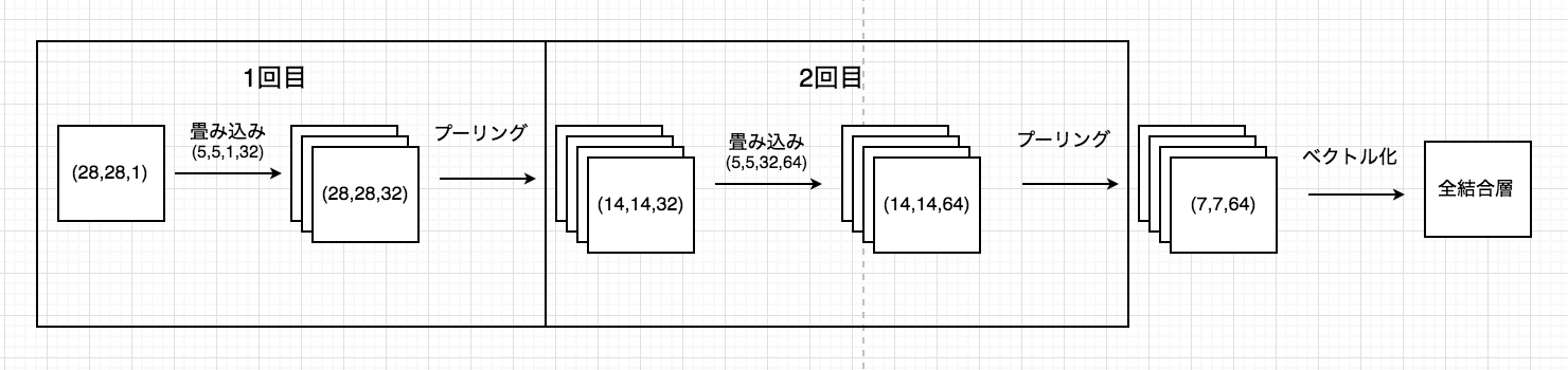
全てネットワークを定義した後に最後に逆伝播させて計算を行っています。

# coding: utf-8

# tensorflowの読み込み
import tensorflow as tf

# データの読み込み
from tensorflow.examples.tutorials.mnist import input_data
mnist = input_data.read_data_sets('MNIST_data',one_hot=True)

# interactiveセッションを起動
sess = tf.InteractiveSession()

# x, y_のplaceholderを定義
x = tf.placeholder(tf.float32,shape=[None,784])
y_ = tf.placeholder(tf.float32,shape=[None,10])

# 関数を定義
## 重みの初期化処理関数
def weight_variable(shape):
    # 正規分布の左右を切り取ったもので初期化
    initial = tf.truncated_normal(shape,stddev=0.1)
    return tf.Variable(initial)


## バイアスの初期化処理関数
def bias_variable(shape):
    initial = tf.constant(0.1,shape=shape)
    return tf.Variable(initial)


## 2次元の畳見込み処理関数(ストライド1, ゼロパディング)
def conv2d(x, W):
    return tf.nn.conv2d(x,W,strides=[1,1,1,1],padding='SAME')


## プーリング関数
def max_pool_2x2(x):
    return tf.nn.max_pool(x,ksize=[1,2,2,1],strides=[1,2,2,1],padding='SAME')


# 1回目
## 1回目の畳み込みで用いるW(重み付け値)
## ([width, height, input, filters] 28×28の画像1(input)枚に対して5(width)×5(height)の32種類(filters)の畳み込みフィルターでそれぞれ畳み込み)
W_conv1 = weight_variable([5,5,1,32])
## 1回目の畳み込みで用いるb(バイアス)
b_conv1 = bias_variable([32])
# 入力の画像。畳み込みを行うためにテンソルに戻している。
# -1はをreshapeに設定することで実行時に動的に値が決まる
x_image = tf.reshape(x, [-1,28,28,1])
# 1回目の畳み込み
h_conv1 = tf.nn.relu(conv2d(x_image,W_conv1) + b_conv1)
# 1回目のプーリング
h_pool1 = max_pool_2x2(h_conv1)


# 2回目
## 2回目の畳み込みで用いるW(重み付け値)
## ([width, height, input, filters] 14×14の画像32枚に対して5×5の64種類の畳み込みフィルターでそれぞれ畳み込み)
W_conv2 = weight_variable([5,5,32,64])
## 2回目の畳み込みで用いるb(バイアス)
b_conv2 = bias_variable([64])
## 1回目のプーリングで出力されたテンソルを使って2回目の畳み込み
h_conv2 = tf.nn.relu(conv2d(h_pool1, W_conv2) + b_conv2)
## 2回目のプーリング
h_pool2 = max_pool_2x2(h_conv2)


# 全結合層(全ての入力を1つにまとめてsoftmax関数に入力)
## 全結合層で用いるW(重み付け値)
W_fc1 = weight_variable([7*7*64,1024])
## 全結合層で用いるb(バイアス)
b_fc1 = bias_variable([1024])
## 2回目の畳み込みで出力されたh_pool2を2次元のテンソルに変換
h_pool2_flat = tf.reshape(h_pool2,[-1,7*7*64])
## 全結合層での結果を出力
h_fc1 = tf.nn.relu(tf.matmul(h_pool2_flat,W_fc1) + b_fc1)


## DropOut(過学習を抑える処理)
keep_prob = tf.placeholder(tf.float32)
h_fc1_drop = tf.nn.dropout(h_fc1,keep_prob)

## 全結合層へのDropOutで用いるW(重み付け値)
W_fc2 = weight_variable([1024,10])
## 全結合層へのDropOutで用いるb(バイアス)
b_fc2 = bias_variable([10])

# 最終的な予測を出力
y_conv = tf.matmul(h_fc1_drop, W_fc2) + b_fc2


# 最小化したいcross_entropyを定義
cross_entropy = tf.reduce_mean(tf.nn.softmax_cross_entropy_with_logits(y_conv,y_))
# AdamOptimizerを用いた最小化のステップを定義
train_step = tf.train.AdamOptimizer(1e-4).minimize(cross_entropy)

# このあたりはBegginerと同じ
correct_prediction = tf.equal(tf.argmax(y_conv,1),tf.argmax(y_,1))
accuracy = tf.reduce_mean(tf.cast(correct_prediction,tf.float32))
sess.run(tf.initialize_all_variables())

# ミニバッチで学習を実行(50をランダムに取って最適化を50回繰り返す)
for i in range(20000):
    batch = mnist.train.next_batch(50)
    # 100回ごとに経過を出力
    if i%100 == 0:
        train_accuracy = accuracy.eval(feed_dict={x:batch[0],y_:batch[1],keep_prob:1.0})
        print("step %d, training accuracy %g"%(i,train_accuracy))
    train_step.run(feed_dict={x:batch[0],y_:batch[1],keep_prob:0.5})

print("test accuracy %g"%accuracy.eval(feed_dict={x: mnist.test.images, y_:mnist.test.labels, keep_prob: 1.0}))

捕捉

畳み込みニューラルネットワークの理解についてはこちらがとても参考になりました。