This article is an English translation from the original article 干渉計の偏波較正 in Japanese.
Introduction
This article aims to calculate polarization-calibrated Stokes visibilities, $I, Q, U, V$, using correlator outputs, $\left< XX^* \right>, \left< XY^* \right>, \left< YX^* \right>, \left< YY^* \right> $, of linearly polarized feeds $(X, Y)$ such as ALMA.
Symbols and General Formulation
Linear Feeds and D-terms
Let $E_X$ and $E_Y$ the linearly polarized electric fields received at each antenna. Antenna optics and receiving systems may have cross talks and the correlator-input signals, $X$ and $Y$ would be given as
X = G_X (E_X + D_X E_Y), \\
Y = G_Y (E_Y + D_Y E_X).
Here, the complex numbers $D_X$ and $D_Y$ are D-terms that describes leakages of $E_Y \rightarrow X$ and $E_X \rightarrow Y$ respectively.
The correlator outputs four correlation pairs of
$\left< X_j X^*_i\right>,$
$\left< X_j Y^*_i\right>,$
$\left< Y_j X^*_i\right>,$
$\left< Y_j Y^*_i\right>.$
where $i, j$ stand for antenna index which relate to the baseline index, $k$, with the Canonical ordering.
Relation between Stokes Parameter and Correlation Pairs
The Stokes parameters, $\boldsymbol{S} = (I, Q, U, V)$, express the polarized source visibilities. $I$ stands for the total flux density, $Q, U$ for linear polarization components, and $V$ for circular polarization one. The Stokes parameters relate to the correlation pairs as
\boldsymbol{X} = D P \boldsymbol{S}, \tag{1.2}
where
\boldsymbol{S} = \left(
\begin{array}{c}
I \\
Q \\
U \\
V \\
\end{array}
\right), \
\boldsymbol{X} = \left(
\begin{array}{c}
\left< XX^* \right> / ( G^j_X G^{i*}_X ) \\
\left< XY^* \right> / ( G^j_X G^{i*}_Y ) \\
\left< YX^* \right> / ( G^j_Y G^{i*}_X ) \\
\left< YY^* \right> / ( G^j_Y G^{i*}_Y ) \\
\end{array}
\right).
Here, the matrices $D$ and $P$ are given as
D =
\left(
\begin{array}{cccc}
1              & D^{i*}_X        & D^j_X           & D^j_X D^{i*}_X \\
D^{i*}_Y       & 1               & D^j_X D^{i*}_Y  & D^j_X          \\
D^j_Y          & D^j_Y D^{i*}_X  & 1               & D^{i*}_X       \\
D^j_Y D^{i*}_Y & D^j_Y           & D^{i*}_Y        & 1              \\
\end{array}
\right) \\
P =
\left(
\begin{array}{cccc}
1 &  \cos 2\psi  &  \sin 2\psi & 0 \\
0 & -\sin 2\psi  &  \cos 2\psi & i \\
0 & -\sin 2\psi  &  \cos 2\psi & -i \\
1 & -\cos 2\psi  & -\sin 2\psi & 0 \\
\end{array}
\right).
Parallactic angle
In the matrix $P$, $\psi$ stands for the orientation of $X$-polarization feed with respect to the north. This is given by $\psi = {\rm PA} + {\rm BandPA}$, where BandPA stands for the orientation of the X-feed with respect to the EL axis. PA is the parallactic angle which describes the orientation of EL axis with respect to the north. In the case of ALT-AZ mount antenna, the parallactic angle changes while tracking the source.
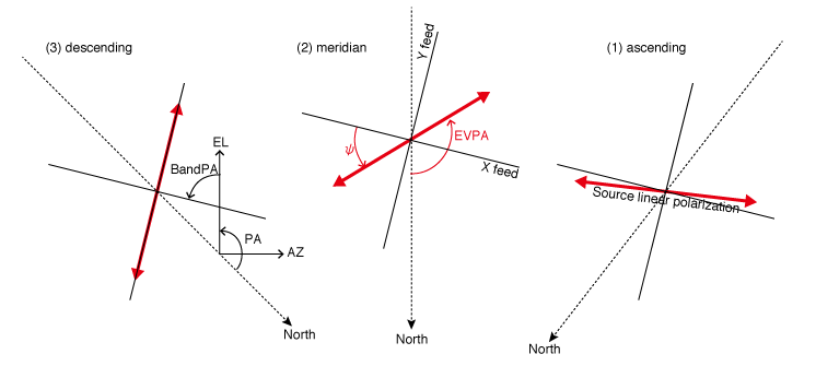
The figure illustrates the source EVPA (Electric Vector Position Angle, in read arrow), PA, and $\psi$ in the ALT-AZ coordinate. PA change by diurnal motion is given by the Python code:
cos_lat, sin_lat = math.cos(lat), math.sin(lat)
PA = np.arctan2( -cos_lat* np.sin(az),  (sin_lat* np.cos(el) - cos_lat* np.sin(el)* np.cos(az)) )
where lat, az, el are latitude, azimuth, and elevation angles of the antenna.
Calibration Methods
Here I summarize the equation (1.2). We want to obtain the Stokes parameter $\boldsymbol{S}$ using the correlation pairs
$\left< X_j X^*_i\right>$,
$\left< X_j Y^*_i\right>$,
$\left< Y_j X^*_i\right>$,
$\left< Y_j Y^*_i\right>$
that we have.
The matrix $P$ is already given, while $D$ and $\boldsymbol{G}$ are unknown. We have to determine them via calibration processes. After $D$ and $\boldsymbol{G}$ are determined, we can solve for $\boldsymbol{S}$ as
\boldsymbol{S} = P^{-1} D^{-1} \boldsymbol{X}. \tag{1.3}
Here inverse matrices $D^{-1}$ and $P^{-1}$ are given by
D^{-1} = \frac{1}{(1 - D^j_X D^j_Y)(1 - D^{i*}_X D^{i*}_Y)}
\left(
\begin{array}{cccc}
1              & -D^{i*}_X       & -D^j_X          & D^j_X D^{i*}_X \\
-D^{i*}_Y      & 1               & D^j_X D^{i*}_Y  & -D^j_X         \\
-D^j_Y         & D^j_Y D^{i*}_X  & 1               & -D^{i*}_X      \\
D^j_Y D^{i*}_Y & -D^j_Y          & -D^{i*}_Y       & 1              \\
\end{array}
\right), \\
P^{-1} = \frac{1}{2}
\left(
\begin{array}{cccc}
1          &  0           &  0          & 1 \\
\cos 2\psi & -\sin 2\psi  & -\sin 2\psi & -\cos 2\psi \\
\sin 2\psi &  \cos 2\psi  &  \cos 2\psi & -\sin 2\psi \\
0          & -i           &  i          & 0 \\
\end{array}
\right).
How to calibrate $D$ and $\boldsymbol{G}$?
Their derivations are described in this article.