概要

Pythonの機械学習系ライブラリscikit-learnの基本的な使い方と、便利だなと思ったものを記載しました。

類似記事は沢山ありますが、自分自身の整理のためにもまとめてみました。
これから、scikit-learnを利用する人にとって、役立つ記事になったら嬉しいです。

準備

Pythonインストール： Windows / Mac
scikit-learnインストール

pip install scikit-learn

公式サイト

基本的なモデルクラスの使い方

モデルインスタンス生成
fitさせる (学習)
predictする (予測)

scikit-learnはAPIが統一されていて、とてもわかりやすいです。

SVMの例

import文

svm.py

from sklearn.svm import SVC
from sklearn.model_selection import train_test_split
import numpy as np
import pandas as pd

データセットを適当に作成

svm.py

# class: 0
df_a = pd.DataFrame({'x1': np.random.randn(100),
                     'x2': np.random.randn(100),
                     'y' : 0})
# class: 1
df_b = pd.DataFrame({'x1': np.random.randn(100) + 5,
                     'x2': np.random.randn(100) + 3,
                     'y' : 1})
df = df_a.append(df_b)

# トレーニングデータとテストデータに分割
X_train, X_test, y_train, y_test = \
    train_test_split(df[['x1','x2']], df['y'], test_size=0.2)

モデルクラスを利用した学習と予測

svm.py

# 1. モデルインスタンス生成
clf = SVC()

# 2. fit 学習
clf.fit(X_train, y_train)

# 3. predict 予測
y_pred = clf.predict(X_test)

SVMによる予測結果がy_predに格納されます。

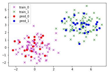
回帰も分類も生成するモデルのクラスを変えるだけで、様々なモデルを簡単に構築できます。

便利機能

ダミー変数変換

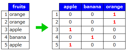
LabelEncoder と OneHotEncoder

LabelEncoder : 文字を数値に変換
OneHotEncoder :　数値をダミー変数に変換

合わせると、カテゴリカル変数をダミー変数に置き換えることができる。

class_report.py

from sklearn.preprocessing import OneHotEncoder, LabelEncoder

le = LabelEncoder()
oe = OneHotEncoder()
en = le.fit_transform(['orange','orange','apple','banana','apple'])
print(oe.fit_transform(en.reshape(-1, 1)).toarray())

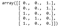
イメージ

※次のバージョン(v0.20)でCategoricalEncoderが追加されるようです！
CategoricalEncoder

データ分割

train_test_split

学習用データとテストデータを分けるため、データセットをランダムに分割する。

data_split.py

from sklearn.model_selection import train_test_split

X_train, X_test, y_train, y_test = \
       train_test_split(X, y, test_size=0.2, random_state=0)

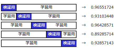
交差検証(CV)

cross_val_score

k分割交差検証法の結果を出力。

cross_val.py

from sklearn.model_selection import cross_val_score

clf = LogisticRegression()

# 5等分の交差検証
print(cross_val_score(clf, X, y, cv=5))

>> array([ 0.96551724,  0.93103448,  0.96428571,  0.89285714,  0.92857143])

イメージ

ハイパーパラメータ選択

GridSearchCV

グリッドサーチと交差検証を同時に行う。

探索したいハイパーパラメータをdict形式で定義し、GridSearchCVの引数として渡す。
GridSearchCVのfitは、交差検証で最も良いスコアとなるハイパーパラメータで学習してくれる。
便利すぎでしょ!!

grid_cv.py

from sklearn.model_selection import GridSearchCV
from sklearn.ensemble import RandomForestClassifier

# 探索したハイパーパラメータ
param_grid = {'n_estimators': [2, 5, 10],
              'max_depth': [2, 5]}

grid_search = GridSearchCV(RandomForestClassifier(random_state=0), param_grid, cv=5)

# 最適なパラメータで学習
grid_search.fit(X_train, y_train)

print('test_score : {}'.format(grid_search.score(X_test, y_test)))
print('best_params : {}'.format(grid_search.best_params_))

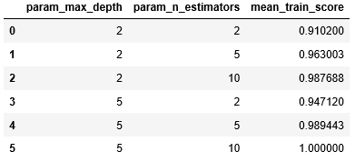
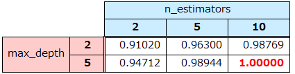
# 各パラメータのCV平均スコア
display(display(pd.DataFrame(grid_search.cv_results_)\
       [['param_max_depth', 'param_n_estimators', 'mean_train_score']]))

結果

>> test_score : 0.9444444444444444
>> best_params : {'max_depth': 5, 'n_estimators': 10}

イメージ

パイプライン

Pipeline

一連の処理ステップをEstimatorとしてまとめることができる。
① 標準化 → ② 次元削減 → ③ ランダムフォレストで学習
の流れを、グリッドサーチ＋CVで検証する場合の例を記載。

グリッドサーチの探索パラメータはPipelineで指定した任意の文字列に”__”(アンダースコア2つ)を付けて指定。

Pipelineで指定できるEstimatorは最後のもの以外はtransformメソッドが定義されている必要がある。

pipe_line.py

from sklearn.pipeline import Pipeline
from sklearn.preprocessing import StandardScaler
from sklearn.decomposition import PCA

# パイプライン生成
pipe = Pipeline([('scaler', StandardScaler()),
                 ('pca', PCA()),
                 ('rf', RandomForestClassifier(random_state=0))])

# グリッドサーチ用の探索ハイパーパラメータ設定
param_grid = {
    'pca__n_components': [2, 3, 4],
    'rf__n_estimators' : [2, 10, 100],
    'rf__max_depth' : [10, 100, 1000]
}

grid_search = GridSearchCV(pipe, param_grid , cv=5)
grid_search.fit(X_train, y_train)

print('test_score : {}'.format(grid_search.score(X_test, y_test)))
print('best_params : {}'.format(grid_search.best_params_))

結果

>> test_score : 0.9722222222222222
>> best_params : {'pca__n_components': 2, 'rf__max_depth': 10, 'rf__n_estimators': 10}

(標準化+PCAがランダムフォレストに適するかはスルーで)

make_pipeline

各ステップに明示的に名前をつけなくても、自動でクラス名の小文字によって名前を付けてくれる。

make_pipeline.py

from sklearn.pipeline import make_pipeline

pipe = make_pipeline(StandardScaler(), PCA(), RandomForestClassifier(random_state=0))

param_grid = {
    'pca__n_components': [2, 3, 4],
    'randomforestclassifier__n_estimators' : [2, 10, 100],
    'randomforestclassifier__max_depth' : [10, 100, 1000]
}

特徴量選択

SelectKBest

特徴量をk個に絞る。

分類 ( score_func=f_classif ) はANOVAによって、関連が高い特徴量を選択している。
回帰 ( score_func=f_regression ) は相関係数によって、関連が高い特徴量を選択している。

from sklearn.feature_selection import SelectKBest, f_regression

sb= SelectKBest(score_func=f_regression, k=10) 
sb.fit(X, y)
X_sb = sb.transform(X)

SelectPercentile

特徴量を割合で指定して絞る。

from sklearn.feature_selection import SelectPercentile

sp = SelectPercentile(percentile=50)
sp.fit(X, y)
X_sp = sp.transform(X)

評価(分類)

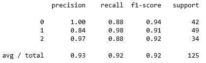
classification_report

分類問題の評価基準であるprecision(適合率)、recall(再現率)、f1-score(F値)、support(実際のサンプル数)を出力。

class_report.py

from sklearn.metrics import classification_report

classification_report(y_true, y_pred)

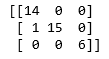
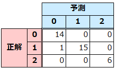
confusion_matrix

混同行列を出力

confusion_matrix.py

from sklearn.metrics import confusion_matrix

print(confusion_matrix(y_test, y_pred))

イメージ

評価(回帰)

mean_squared_error

平均二乗誤差を出力。

MSE = \frac{1}{n} \ \sum_{i=1}^{n} (f_{i}-y_{i})^2 \\

mse.py

from sklearn.metrics import mean_squared_error

# RMSE
np.sqrt(mean_squared_error(y_test, y_pred))

>> 0.62519679744672363

文章のTF-IDFベクトル変換

Tfidfvectorizer

文章内における単語の重要度を数値化するTF-IDF法の結果を出力。

tf-idf.py

from sklearn.feature_extraction.text import TfidfVectorizer

tf_idf = TfidfVectorizer()
X = tf_idf.fit_transform(['Hello mom.',
                          'I am tired.',
                          'I am lazy.',])
print(X.toarray())

結果

[[ 0.          0.70710678  0.          0.70710678  0.        ]
 [ 0.60534851  0.          0.          0.          0.79596054]
 [ 0.60534851  0.          0.79596054  0.          0.        ]]

データセット

データセットがついている。
とりあえず、何かデータセットが必要な時に便利。

API	説明
load_boston	米国ボストン市郊外における地域別の住宅価格	回帰
load_iris	3 種類の品種のアヤメのがく片、花弁の幅および長さ	分類
load_diabetes	糖尿病患者の検査数値と1年後の疾患進行状況	回帰
load_digits	0~9の手書き文字の8×8画像	分類
load_linnerud	成人男性の生理学的特徴と運動能力	回帰
load_wine	3種類のワインの科学的特徴	分類
load_breast_cancer	乳がんの診断結果	分類

データの取得

from sklearn.datasets import load_wine

# ワインデータ取得
data, target = load_wine(return_X_y=True)

おわり

誤った記載がありましたら、ご指摘いただけたら嬉しいです。
まだまだ、sklearn使いこなせてないので、ガシガシ使っていきたいです！

機械学習ライブラリ scikit-learnの便利機能の紹介

概要

準備

公式サイト

基本的なモデルクラスの使い方

SVMの例

便利機能

ダミー変数変換

LabelEncoder と OneHotEncoder

データ分割

train_test_split

交差検証(CV)

cross_val_score

ハイパーパラメータ選択

GridSearchCV

パイプライン

Pipeline

make_pipeline

特徴量選択

SelectKBest

SelectPercentile

評価(分類)

classification_report

confusion_matrix

評価(回帰)

mean_squared_error

文章のTF-IDFベクトル変換

Tfidfvectorizer

データセット

おわり