※ 2020/12/28 デプロイの節を追加
はじめに
この記事ではstreamlitでいくつかアプリケーションを作成し、streamlitに入門することを目的とします。
streamlitを用いて、プロトタイプアプリを簡単に作成できるようになれればと思います。
repository: https://github.com/irisu-inwl/streamlit-tutorial
動作確認環境: windwos10, docker for windows
- この記事でやること

- streamlitでアプリケーションを作るために利用できそうなメソッド群の紹介
- 機械学習・データ分析アプリケーションのプロトタイプの作成
- この記事で取り扱わないこと

- 機械学習アルゴリズムの解説
- データサイエンス部分の解説
準備
streamlit環境をdockerで用意します。
docker build --tag streamlit-base .
docker run -itd -p 8080:8080 --name streamlit-tutorial streamlit-base
streamlitでwidgeを配置する。
widgetを次のように簡単に書くことが出来、インタラクティブなアプリケーションを実装できます
ソース: https://github.com/irisu-inwl/streamlit-tutorial/blob/main/src/widget.py
- 環境準備
docker run -itd -p 8080:8080 -v <自分のsrcディレクトリ>:/opt/streamlit/src/ --name streamlit-tutorial streamlit-base streamlit run src/widget.py
localhost:8080にアクセスすることでアプリケーションを確認できます。
デモ:
— いりす (@irisuinwl) November 18, 2020
以下にコードで利用した細かい機能を紹介していきます。
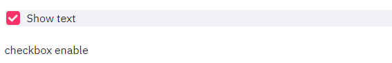
チェックボックス
下記のコードでチェックボックスを配備できます。
st.checkboxメソッドの引数にラベル、返り値に状態が入ります。
# checkbox
checkbox_state = st.checkbox('Show text')

if checkbox_state:
    st.write('checkbox enable')

ボタン
ボタンウィジェットを下記コードで配置します。
チェックボックス同様に、引数にラベル、返り値に状態が入ります。
# button
button_state = st.button('Say hello')
if button_state:
    st.write('Why hello there')
else:
    st.write('Goodbye')


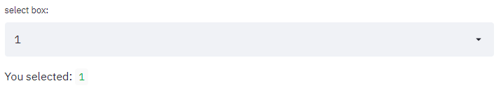
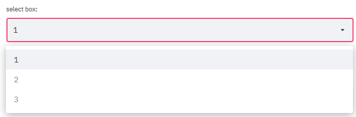
セレクトボックス
セレクトボックスをst.selectboxで配備できます。
第一引数にラベル、第二引数に選択する範囲を指定できます。
# selectbox
option = st.selectbox(
    'select box:',
    [1, 2, 3]
)

st.write('You selected: ', option)
インプットボックス
文字入力を行うインプットボックスを配置します。
# inputbox
title = st.text_input('inputbox', 'おはよう')
st.write('inputbox:', title)
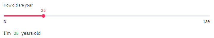
スライダー
スライダーを配置します。
# slider
age = st.slider('How old are you?', 0, 130, 25)
st.write("I'm ", age, 'years old')
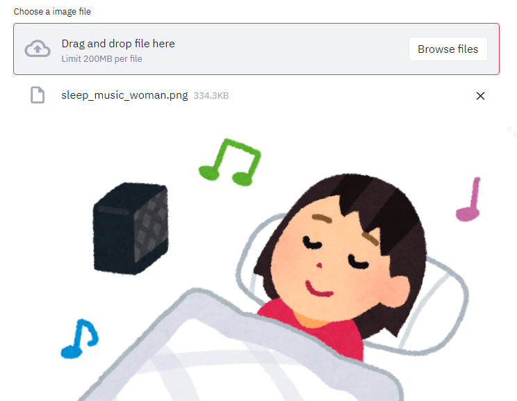
ファイルアップロード
画像をドラッグアンドドロップしてアップロードする処理がst.file_uploaderで可能となります。
下記処理で、画像がアップロードされればuploaded_fileが存在するのでifブロックに入ります。
# file upload
from PIL import Image
import io
uploaded_file = st.file_uploader('Choose a image file')

if uploaded_file is not None:
    image = Image.open(uploaded_file)
    img_array = np.array(image)
    st.image(
        image, caption='upload images',
        use_column_width=True
    )
キャッシュ処理
streamlitではイベントが発火する度、コードを再実行します。
cf: https://docs.streamlit.io/en/stable/main_concepts.html#app-model
そのため、巨大なデータを読み込んだり、計算時間のかかる処理を実行すると、イベント発火のたびに描画に時間がかかってしまいます。
そこで、streamlitではキャッシュを利用することによって、処理を効率化します。
下記例では、waitを掛けるメソッドに対して、プログレスバーを表示する処理で、キャッシュを使った場合と使わなかった場合を見てます。
import time

import streamlit as st


@st.cache
def progress_cache(i):
    time.sleep(0.05)


def progress_no_cache(i):
    time.sleep(0.05)


def view_bar(func):
    # Add a placeholder
    latest_iteration = st.empty()
    bar = st.progress(0)

    for i in range(100):
        # Update the progress bar with each iteration.
        latest_iteration.text(f'Iteration {i+1}')
        bar.progress(i + 1)
        func(i)


st.title('Cache example')
st.write('Starting a long computation with cache...')
view_bar(progress_cache)

st.write('Starting a long computation without cache...')
view_bar(progress_no_cache)

st.write('...and now we\'re done!')
— いりす (@irisuinwl) November 21, 2020
データ可視化
ランダムデータやアイリスデータを使ってデータの可視化をしてみます。
ソース: https://github.com/irisu-inwl/streamlit-tutorial/blob/main/src/visualization.py
docker run -itd -p 8080:8080 -v <自分のsrcディレクトリ>:/opt/streamlit/src/ --name streamlit-tutorial streamlit-base streamlit run src/visualization.py
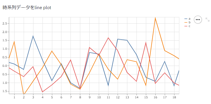
LinePlot
@st.cache
def load_time_series_data():
    """
    ランダムに時系列データを生成する。
    """
    chart_data = pd.DataFrame(
        np.random.randn(20, 3),
        columns=['a', 'b', 'c']
    )
    return chart_data

st.write('時系列データをline plot')
chart_data = load_time_series_data()
st.line_chart(chart_data)
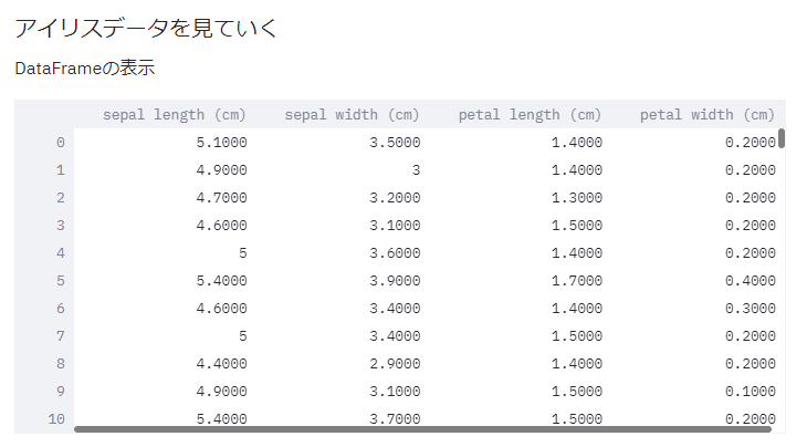
DataFrame表示
DataFrameもst.writeで画面描画することが出来ます。
@st.cache
def load_iris_data():
    """
    データ読み込み, cacheにして最適化を行う
    """
    iris_data = load_iris()
    df = pd.DataFrame(iris_data.data, columns=iris_data.feature_names)
    labels = iris_data.target_names[iris_data.target]
    return df, labels

st.write('### アイリスデータを見ていく')
df, labels = load_iris_data()

st.write('DataFrameの表示')
st.write(df)
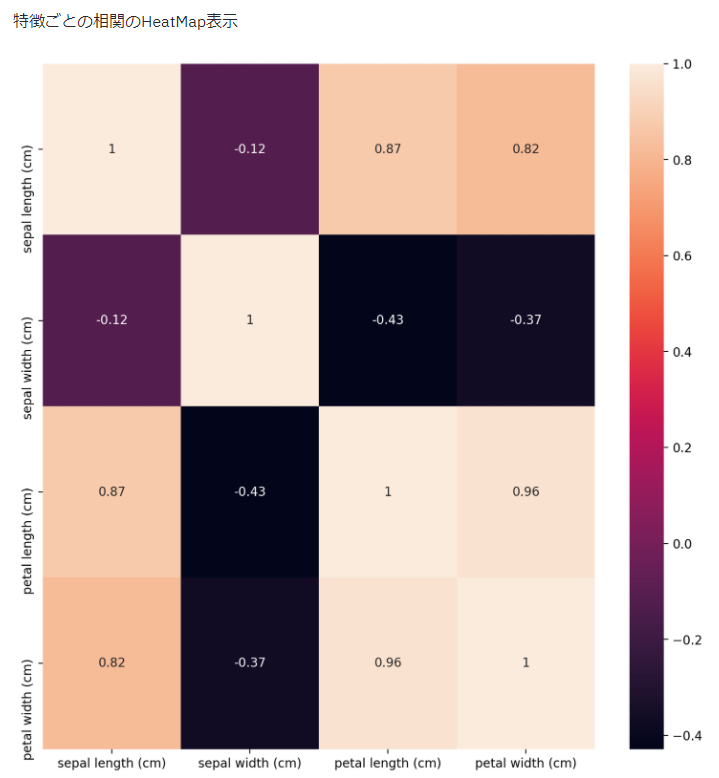
相関ヒートマップ
seabornやmatplotlibをwrapして表示できます。
def show_heatmap(df):
    """
    各特徴の相関ヒートマップをみる
    """
    fig, ax = plt.subplots(figsize=(10,10))
    sns.heatmap(df.corr(), annot=True, ax=ax)
    st.pyplot(fig)

st.write('特徴ごとの相関のHeatMap表示')
show_heatmap(df)
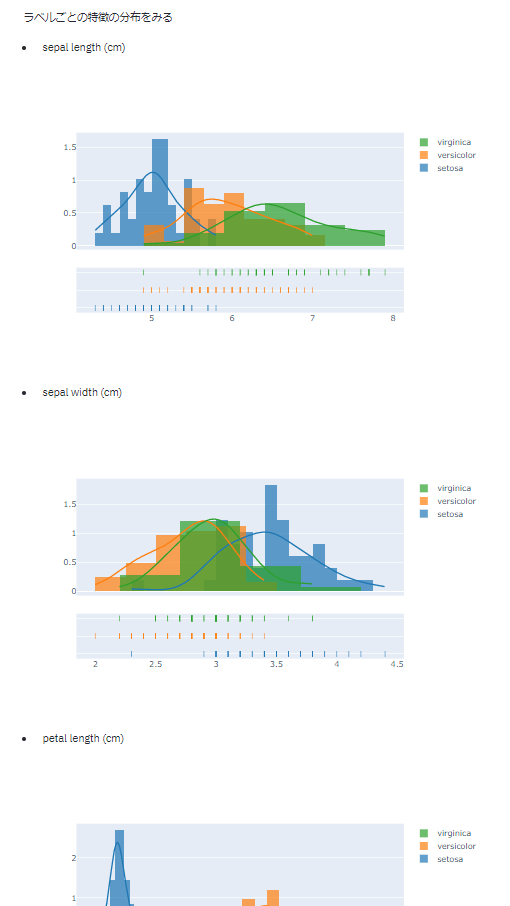
特徴とラベルごとに分布を出す
def show_distplot(df, labels):
    """
    それぞれの特徴について、各ラベルごとの分布を見る
    """
    for column in df.columns:
        st.write(f'- {column}')
        series = df[column]
        target_names = list(set(labels))
        hist_data = [series[labels == name] for name in target_names]
        fig = ff.create_distplot(
            hist_data, target_names, bin_size=[.1, .25, .5])
        st.plotly_chart(fig, use_container_width=True)

st.write('ラベルごとの特徴の分布をみる')
show_distplot(df, labels)
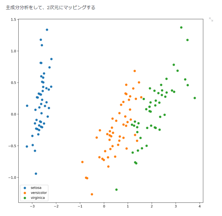
PCAで2次元にマッピング
@st.cache(allow_output_mutation=True)
def fit_transform_pca(df):
    """
    主成分分析した結果の第二主成分ベクトルを可視化した結果を得る
    """
    pca = PCA(n_components=2)
    X = pca.fit_transform(df)
    return X

def show_scatter2d(X, labels):
    fig, ax = plt.subplots(figsize=(10,10))
    target_names = list(set(labels))
    for i, target in enumerate(target_names):
        X_ = X[labels == target]
        x = X_[:, 0]
        y = X_[:, 1]
        ax.scatter(x, y, cmap=[i]*len(X_), label=target)

    ax.legend()
    st.pyplot(fig)

st.write('主成分分析をして、2次元にマッピングする')
df_pca = fit_transform_pca(df)
show_scatter2d(df_pca, labels)
画像分類アプリを作る
kerasのpretrainedモデルを使って、画像分類アプリを作ります。
コード: https://github.com/irisu-inwl/streamlit-tutorial/blob/main/src/image_clf.py
widget.pyで紹介したファイルアップロードを使い画像を読込、kerasのpretrained Xceptionモデルを読みだして予測するコードを以下のように書きます。
cf: https://keras.io/ja/applications/#xception
st.set_option('deprecation.showfileUploaderEncoding', False)


@st.cache(allow_output_mutation=True)
def load_model():
    """
    Xceptionモデルをloadする。
    """

    model = Xception(include_top=True, weights='imagenet', input_tensor=None, input_shape=None, pooling=None, classes=1000)

    return model


def preprocessing_image(image_pil_array: 'PIL.Image'):
    """
    予測するためにPIL.Imageで読み込んだarrayを加工する。
    299×299にして、pixelを正規化

    cf: https://keras.io/ja/applications/#xception
    """

    image_pil_array = image_pil_array.convert('RGB')
    x = image.img_to_array(image_pil_array)
    x = np.expand_dims(x, axis=0)
    x = preprocess_input(x)

    return x


model = load_model()

st.title('画像分類器')

st.write("pretrained modelを使って、アップロードした画像を分類します。")

uploaded_file = st.file_uploader('Choose a image file')

if uploaded_file is not None:
    image_pil_array = Image.open(uploaded_file)
    st.image(
        image_pil_array, caption='uploaded image',
        use_column_width=True
    )

    x = preprocessing_image(image_pil_array)
    result = model.predict(x)

    predict_rank = decode_predictions(result, top=5)[0]
    st.write('機械学習モデルは画像を', predict_rank[0][1], 'と予測しました。')

    st.write('#### 予測確率@p5')
    df = pd.DataFrame(predict_rank, columns=['index', 'name', 'predict_proba'])
    st.write(df)
    df_chart = df[['name', 'predict_proba']].set_index('name')
    st.bar_chart(df_chart)
また、モデルのdownloadをアプリ起動ごとするのは面倒なので、dockerfileにダウンロードスクリプトを仕込みます。
- download_model.py
from tensorflow.keras.applications.xception import Xception, preprocess_input, decode_predictions

model = Xception(include_top=True, weights='imagenet', input_tensor=None, input_shape=None, pooling=None, classes=1000)
Dockerfileで呼び出し処理を書き、build時にモデルのダウンロードを行います。
RUN python src/download_model.py
以下のようなアプリが出来上がりました。
— いりす (@irisuinwl) November 20, 2020
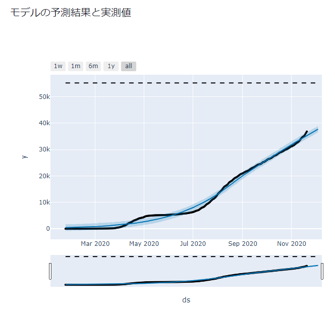
時系列分析アプリを作る
Facebookの時系列分析ライブラリprophetと東京都COVID-19のデータを使い、東京都COVID-19感染者数を時系列分析するアプリを作ります。
モデルは、簡単に考えるため、SIモデル(SIRモデルからRを除いたもの)を用います、つまり、感染者総数をロジスティック曲線でfittingすることを考えます。
モデルの学習と予測を行います。
dsに日付、yに値が入ったDataFrameに対して、fitで学習、predictで予測が出来ます。
@st.cache(allow_output_mutation=True)
def fit_and_forecast(df: 'pd.DataFrame', periods:int = 14):
    """
    与えられたDataFrameに対して、prophetのmodelと予測結果を返す
    """
    model = Prophet(growth='logistic')
    model.fit(df)
    future = model.make_future_dataframe(periods=periods)
    future['cap'] = df.iloc[0].cap
    forecast = model.predict(future)
    return model, forecast

df = load_data('data/data.json')

st.write('### 直近の感染者数')
st.write(df.tail())

prophet_df = df[['日付', '感染者総数']].rename(columns={'日付':'ds', '感染者総数':'y'})
prophet_df['cap'] = prophet_df.iloc[-1].y*1.5

model, forecast = fit_and_forecast(prophet_df)
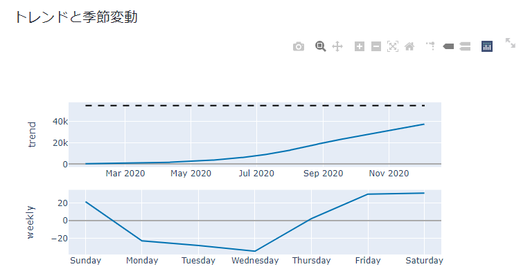
- モデルの予測値と実測値、トレンドと季節変動、変化点の表示
学習・予測した結果とモデルの推定したトレンドや季節変動、変化点を表示します。
st.write('### モデルの予測結果と実測値')
fig = plot_plotly(model, forecast)
st.plotly_chart(fig, use_container_width=True)
st.write('### トレンドと季節変動')
fig = plot_components_plotly(model, forecast)
st.plotly_chart(fig, use_container_width=True)
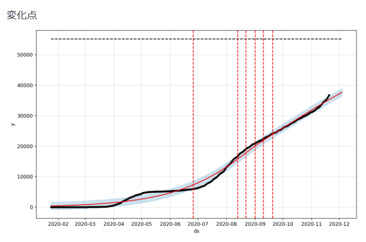
st.write('### 変化点')
fig = model.plot(forecast)
add_changepoints_to_plot(fig.gca(), model, forecast)
st.pyplot(fig)
GCPにデプロイしよう!
せっかく作ったアプリなので、GCPにデプロイします。
手順としては、StreamlitアプリケーションをGCP(GAE)にデプロイする方法の記事とほぼ同じです。
ここでは、試行錯誤した結果を記載します。
(失敗)cloud runでデプロイしてみる!
cloud runでデプロイすると、アプリを開くと以下の画面が出てきて動作しません。
ぐぐってみると、公式のissueに「websocketで永続的に通信してるからサーバーレスみたいなインフラにデプロイは無理っぽいよ」とありました。
https://github.com/streamlit/streamlit/issues/484
なので、GCEかGKEかGAEを使えとのことです。
GAE custom modeでデプロイしてみる!
app.yamlファイルを書いてgcloud app deployをするだけです。
ただ、今回のコードは色々大きいので、VM_DISK_FULLとなってしまったので、以下のリソース設定をapp.yamlに追加してます。
runtime: custom
env: flex

resources:
  cpu: 1
  memory_gb: 2
  disk_size_gb: 20
おわり
以上になります。
streamlit便利! 最高! というお気持ちが伝われば良いかなーと。
コード中にバグや不備があったらコメントやissueお願いします ![]()
参考:
-
https://docs.streamlit.io/en/stable/getting_started.html
- 公式チュートリアルが豊富なのでここを見ればほぼOKです。
- https://docs.streamlit.io/en/stable/api.html
-
https://docs.streamlit.io/en/stable/caching.html
- streamlitを使った様々なキャッシュの利用方法が載ってます。
- https://facebook.github.io/prophet/docs/quick_start.html
-
https://medium.com/katanaml/covid-19-growth-modeling-and-forecasting-with-prophet-2ff5ebd00c01
- prophetによるモデリングはこちらの記事を参考にしました。
- https://keras.io/ja/