はじめに
定番のGANs(pix2pix)線画着彩を、無料のGoogle Colabでやってみました。
教師データが大きく、また学習時間も長いので、Colabでやるには多少工夫が必要です。
pix2pixの説明は、他の方の分かりやすい記事を見て頂くとよいかと思います。
先にU-Netを理解してからだと、pix2pixの理解が早いと思います。
https://qiita.com/koshian2/items/603106c228ac6b7d8356
https://qiita.com/mine820/items/36ffc3c0aea0b98027fd
事前準備
美少女イラストを収集・厳選・加工し、線画と着彩のデータセットを用意します(以下参考)。
https://www.mathgram.xyz/entry/scraping/pixiv
https://qiita.com/mo-do/items/c7d53507f23f72daea69
https://qiita.com/pashango2/items/145d858eff3c505c100a
npyファイルでGoogle Diveにアップします(ディレクトリ構成はソースコード参照)。
今回は128x128のサイズで3万枚を訓練用、6000枚をテスト用としました。
無料の15G枠でも収まるデータ量です(着彩1.8G、線画600M)。
仮にもっと大きいデータを使う場合でも、100G枠で250円/月とリーズナブルです。
ソースコード
Kerasでの実装です。
GPUランタイムで上から順にコピペすれば動きます。
モデルは下記から拝借しています。
https://github.com/eriklindernoren/Keras-GAN/blob/master/pix2pix/pix2pix.py
必要なimportは以下です。
import sys, time, os, json
import numpy as np
import matplotlib.pylab as plt
from PIL import Image
from keras.models import *
from keras.layers import *
from keras.optimizers import *
from google.colab import drive
Google Diveをマウント
drive_root = '/content/drive'
drive.mount(drive_root)
datasets_dir = "%s/My Drive/datasets"%drive_root
train_dir = "%s/My Drive/train/pix128"%drive_root
os.makedirs(train_dir, exist_ok=True)
実行すると認証を求められるので、認証コードを入れてEnterします。
モデル
生成モデルはU-Netです。
線画を受け取り、同じ大きさの着彩を出力します。
def Unet(img_shape):
    def conv2d(x, filters, bn=True):
        x = Conv2D(filters, 4, strides=2, padding='same')(x)
        x = LeakyReLU(0.2)(x)
        if bn:
            x = BatchNormalization(momentum=0.8)(x)
        return x
    def deconv2d(x, contracting_path, filters, drop_rate=0):
        x = UpSampling2D(2)(x)
        x = Conv2D(filters, 4, padding='same', activation='relu')(x)
        if drop_rate:
            x = Dropout(drop_rate)(x)
        x = BatchNormalization(momentum=0.8)(x)
        return Concatenate()([x, contracting_path])
    img_B = Input(img_shape)
    #エンコーダー
    c1 = conv2d(img_B, 64, False)
    c2 = conv2d(c1, 128)
    c3 = conv2d(c2, 256)
    c4 = conv2d(c3, 512)
    c5 = conv2d(c4, 512)
    c6 = conv2d(c5, 512)
    #中間層
    x = conv2d(c6, 512)
    #デコーダー
    x = deconv2d(x, c6, 512)
    x = deconv2d(x, c5, 512)
    x = deconv2d(x, c4, 512)
    x = deconv2d(x, c3, 256)
    x = deconv2d(x, c2, 128)
    x = deconv2d(x, c1, 64)
    #元サイズ出力
    x = UpSampling2D(2)(x)
    x = Conv2D(img_shape[-1], 4, padding='same', activation='tanh')(x)
    return Model(img_B, x)
識別モデルは単純な畳み込みです。
線画と着彩を受け取り、真偽をPatchGANサイズで出力します。
def Discriminator(img_shape):
    def d_layer(x, filters, bn=True):
        x = Conv2D(filters, 4, strides=2, padding='same')(x)
        x = LeakyReLU(0.2)(x)
        if bn:
            x = BatchNormalization(momentum=0.8)(x)
        return x
    img_A = Input(img_shape)
    img_B = Input(img_shape)
    x = Concatenate()([img_A, img_B])
    #PatchGANのサイズまで畳み込み
    x = d_layer(x, 64, False)
    x = d_layer(x, 128)
    x = d_layer(x, 256)
    x = d_layer(x, 512)
    #0〜1ラベル出力
    x = Conv2D(1, 4, padding='same')(x)
    return Model([img_A, img_B], x)
生成モデルを訓練するための結合モデルです。
def Pix2Pix(gen, disc, img_shape):
    img_A = Input(img_shape)
    img_B = Input(img_shape)
    fake_A = gen(img_B)
    valid = disc([fake_A, img_B])
    return Model([img_A, img_B], [valid, fake_A])
訓練
genとdiscをエポックごとに保存して、稼働時限を超えても最後のエポックから再開します。
img_sizeを大きくする場合、batch_sizeを減らさないとColabのGPUメモリが不足します。
512x512の場合、batch_size=10が限界でした(なお20日以上かかります)。
def train():
    #教師データ
    train_num = 30000
    test_num = 6000
    img_size = 128
    img_shape = (img_size,img_size,3)
    train_A = load_datasets("%s/color.npy"%datasets_dir, train_num+test_num, img_shape)
    train_B = load_datasets("%s/line.npy"%datasets_dir, train_num+test_num, (img_size,img_size))
    #訓練回数
    epochs = 200
    batch_size = 100
    batch_num = train_num // batch_size
    #前回までの訓練情報
    info_path = "%s/info.json"%train_dir
    info = get_json(info_path, lambda: {"epoch":0})
    #PatchGAN
    patch_shape = (img_size//16, img_size//16, 1)
    valid = np.ones((batch_size,) + patch_shape)
    fake = np.zeros((batch_size,) + patch_shape)
    #モデル
    opt = Adam(0.0002, 0.5)
    gen_path = "%s/gen.h5"%train_dir
    disc_path = "%s/disc.h5"%train_dir
    if os.path.isfile(disc_path):
        gen = load_model(gen_path)
        disc = load_model(disc_path)
        print_img(1, gen, train_A, train_B, 0, train_num, "train")
        print_img(1, gen, train_A, train_B, train_num, test_num, "test")
    else:
        gen = Unet(img_shape)
        disc = Discriminator(img_shape)
        disc.compile(loss='mse', optimizer=opt, metrics=['accuracy'])
    disc.trainable = False
    pix2pix= Pix2Pix(gen, disc, img_shape)
    pix2pix.compile(loss=['mse', 'mae'], loss_weights=[1, 100], optimizer=opt)
    #エポック
    for e in range(info["epoch"], epochs):
        start = time.time()
        #ミニバッチ
        for i in range(batch_num):
            #バッチ範囲をランダム選択
            idx = np.random.choice(train_num, batch_size, replace=False)
            imgs_A = train_A[idx].astype(np.float32) / 255
            imgs_B = convert_rgb(train_B[idx]).astype(np.float32) / 255
            #識別訓練
            fake_A = gen.predict(imgs_B)
            d_loss_real = disc.train_on_batch([imgs_A, imgs_B], valid)
            d_loss_fake = disc.train_on_batch([fake_A, imgs_B], fake)
            d_loss = np.add(d_loss_real, d_loss_fake) * 0.5
            #生成訓練
            g_loss = pix2pix.train_on_batch([imgs_A, imgs_B], [valid, imgs_A])
            #ログ
            print("\repoch:%d/%d batch:%d/%d %ds d_loss:%s g_loss:%s" %
                (e+1,epochs, (i+1),batch_num, (time.time()-start), d_loss[0], g_loss[0]), end="")
            sys.stdout.flush()
        print()
        #画像生成テスト
        print_img(e+1, gen, train_A, train_B, 0, train_num, "train")
        print_img(e+1, gen, train_A, train_B, train_num, test_num, "test")
        #重みの保存
        gen.save(gen_path)
        disc.save(disc_path)
        info["epoch"] += 1
        with open(info_path, "w") as f:
            json.dump(info, f)
教師データを全て乗せてしまうとColabのRAMが不足します(512x512の場合)。
なのでmemmapでバッチ単位で読み出します。
def load_datasets(path, train_num, img_shape):
    return np.memmap(path, dtype=np.uint8, mode="r", shape=(train_num,)+img_shape)
学習済みのエポック数はjsonに記録します。
def get_json(json_name, init_func):
    if os.path.isfile(json_name):
        with open(json_name) as f:
            return json.load(f)
    else:
        return init_func()
格納効率から線画はグレースケールで保存しています。
モデルに渡す際はRGBに変換が必要です。
def convert_rgb(train_B):
    return np.array([np.asarray(Image.fromarray(x).convert("RGB")) for x in train_B])
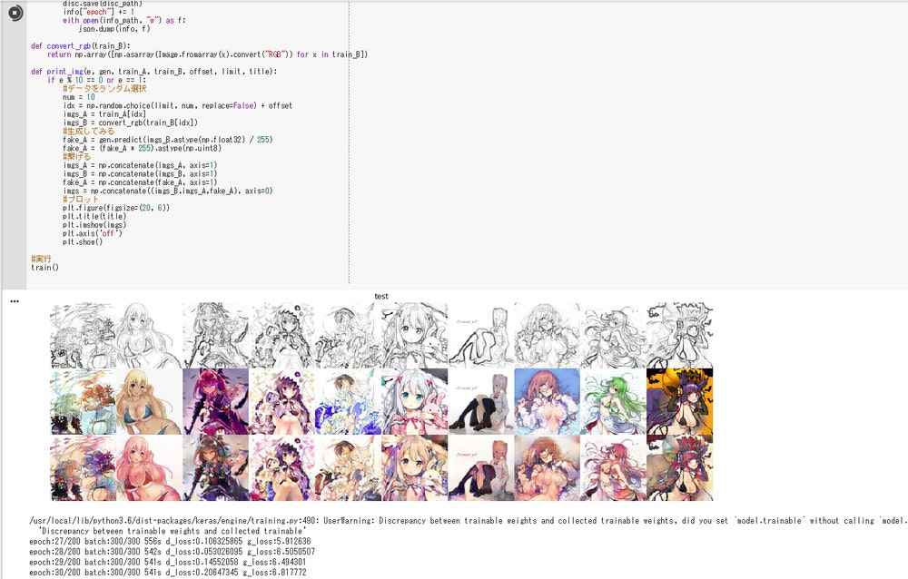
10エポックごとに着彩結果を出力します。
訓練用とテスト用を両方出力して、汎用度を見てみます。
def print_img(e, gen, train_A, train_B, offset, limit, title):
    if e % 10 == 0 or e == 1:
        #データをランダム選択
        num = 10
        idx = np.random.choice(limit, num, replace=False) + offset
        imgs_A = train_A[idx]
        imgs_B = convert_rgb(train_B[idx])
        #生成してみる
        fake_A = gen.predict(imgs_B.astype(np.float32) / 255)
        fake_A = (fake_A * 255).clip(0).astype(np.uint8)
        #繋げる
        imgs_A = np.concatenate(imgs_A, axis=1)
        imgs_B = np.concatenate(imgs_B, axis=1)
        fake_A = np.concatenate(fake_A, axis=1)
        imgs = np.concatenate((imgs_B,imgs_A,fake_A), axis=0)
        #プロット
        plt.figure(figsize=(20, 6))
        plt.title(title)
        plt.imshow(imgs)
        plt.axis('off')
        plt.show()
# 実行
train()
実行結果
1エポック(test)
人物と背景の区別は少しつくようです。
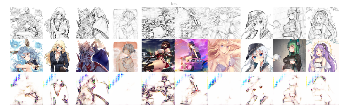
10エポック(test)
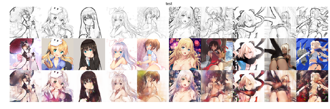
すでになんとなく塗れています。すごい。
26エポック(train)
(ミスって20エポックの画像取れなかった)
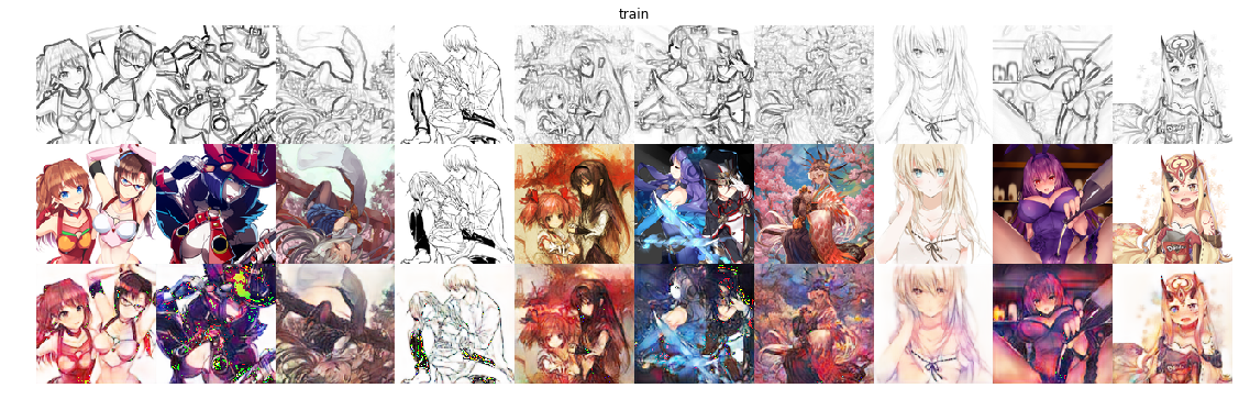
このくらいからtrainデータの色の再現度がかなり高くなってます。
60エポック(test)
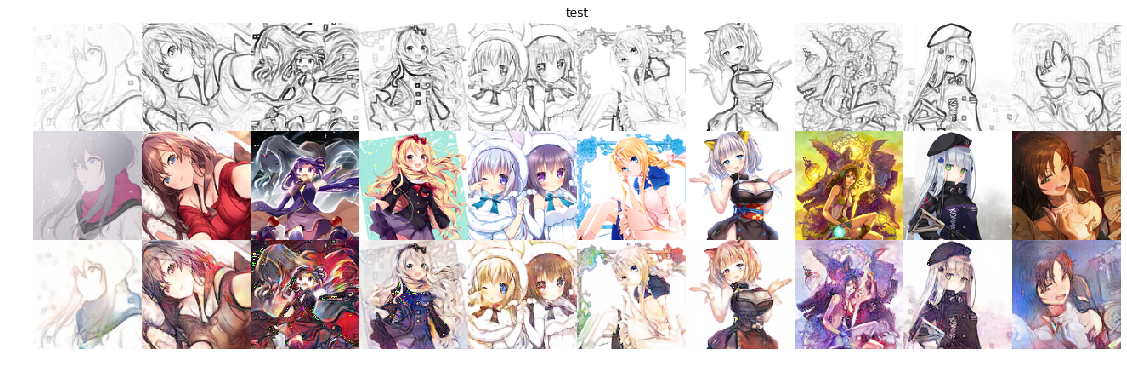
緑の点々は気になりますが、だいぶ色彩豊かになりました。
ルナちゃんの胸元が布になったところに、別の可能性を感じます(センシティブ部位の自動修正など)。
※5/20追記:緑の点々は clip(0) を入れることで解決しました(コード修正済み)。
実行時間
128x128の3万枚で1エポック550秒かかりました(200エポックで約30時間の計算)。
PaintsChainerは512x512を60万枚だと思われますので、この実装とスペックだと約400日でしょうか。
512x512はColab TPUが必要そうです(定評ではGPUの15~30倍のポテンシャル)。
しかしエラーで上手く動かなかったので、チャレンジ中です。
※5/20追記:コメントで指摘いただいておりますが、現行のTPUは複数グラフをサポートしていなかったようです。
おわりに
Google Colabのおかげで無料でも美少女イラストのGANsを楽しめることが分かりました。
それに実装も簡単なので、興味のある人はどんどんやってみることをオススメしたいです。