やったこと
以前紹介したローカルレベルモデルを用いた異常検知で、実際のデータを用いて解析してみました。
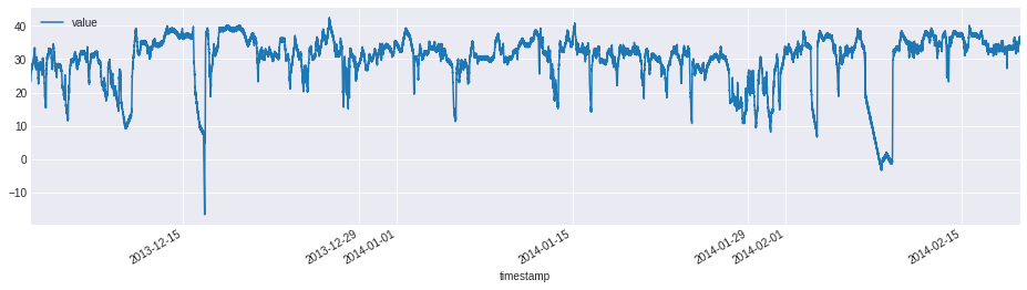
今回用いたデータは異常値を含むデータを多く公開してくれているこちらのNAB(https://github.com/numenta/NAB)というサイトから持ってきた'machine_temperature_system_failure'というもので、機械に備え付けられているセンサーが読み取った機械の内部温度の推移を示したものです。異常値は3ヶ所あって、最初のものは予定されたシャットダウン、2つ目は検知が難しいもので、それが3つ目の異常値に繋がり、機械止まることになったというものです。
(原文)Temperature sensor data of an internal component of a large, industrial mahcine. The first anomaly is a planned shutdown of the machine. The second anomaly is difficult to detect and directly led to the third anomaly, a catastrophic failure of the machine.
ライブラリ
# 基本ライブラリ
import numpy as np
import pandas as pd

# 図形描画ライブラリ
import matplotlib.pyplot as plt
plt.style.use('seaborn-darkgrid')
from matplotlib.pylab import rcParams
rcParams['figure.figsize'] = 15,4

# 統計モデル
import statsmodels.api as sm
データ
data = pd.read_csv('https://raw.githubusercontent.com/numenta/NAB/master/data/realKnownCause/machine_temperature_system_failure.csv')
data.info()
RangeIndex: 22695 entries, 0 to 22694
Data columns (total 2 columns):
timestamp 22695 non-null object
value 22695 non-null float64
dtypes: float64(1), object(1)
memory usage: 354.7+ KB
# change the type of timestamp for plot
data['timestamp'] = pd.to_datetime(data['timestamp'])

# change fahrenheit to c
data['value'] = (data['value'] - 32) * 5/9

# plot
rcParams['figure.figsize'] = 16,4
data.plot(x='timestamp', y='value')
モデリング
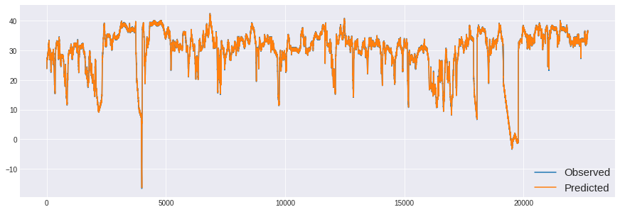
全開の記事と違って、今回はPythonのstatsmodelにあるUnobservedComponentsを用いて推定しました。
mod_local_level = sm.tsa.UnobservedComponents(data.value, 'local level')
res_local_level = mod_local_level.fit()
print(res_local_level.summary())
| sales_ad | dummy_ad | |
|---|---|---|
| 0 | 22.834287 | 0.0 |
| 1 | 26.212849 | 0.0 |
| 2 | 25.638334 | 0.0 |
| 3 | 26.333011 | 0.0 |
| 4 | 25.669880 | 0.0 |
Unobserved Components Results
| Dep. Variable: | value | No. Observations: | 22695 |
|---|---|---|---|
| Model: | local level | Log Likelihood | -19945.532 |
| Date: | Sat, 11 May 2019 | AIC | 39895.065 |
| Time: | 13:39:42 | BIC | 39911.124 |
| Sample: | 0 | HQIC | 39900.287 |
| Covariance Type: | opg |
| coef | std err | z | P>z | [0.025 0.975] |
|---|---|---|---|---|
| sigma2.irregular | 0.0679 | 0.001 | 55.691 | 0.000 |
| sigma2.level | 0.2173 | 0.001 | 233.527 | 0.000 |
| Ljung-Box (Q): | 1673.00 | Jarque-Bera (JB): | 282754.21 |
| Prob(Q): | 0.00 | Prob(JB): | 0.00 |
| Heteroskedasticity (H): | 0.94 | Skew: | 1.38 |
| Prob(H) (two-sided): | 0.01 | Kurtosis: | 20.07 |
rcParams['figure.figsize'] = 15,5
plt.plot(data.value.iloc[1:], label='Observed')
plt.plot(res_local_level.fittedvalues[1:], label='Predicted')
plt.legend(loc='lower right', borderaxespad=0, fontsize=15)
異常検知
sigma = res_local_level.params[0] + res_local_level.params[1]

anomaly_detection = (data.value - res_local_level.fittedvalues[1:])*sigma

plt.plot(anomaly_detection)
plt.title('anomaly detection')
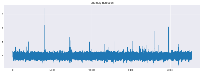
3回あるという異常値をうまく推定できています。ただ閾値をどうするかというところについては、主観的判断になってしまうのでしょうか…。統計的アプローチだとしかたないのかも…。