コンピュータービジョン学び直し — Traditional approach to GANs —

□ イントロ

コンピュータービジョンをさらっと学び直した＠Udemyのでここにメモを残しておく。¹
⇓ アルゴリスムと実装の詳細はこちらを参考にされたい。

• Deep Learning and Computer Vision A-Z™: OpenCV, SSD & GANs: Become a Wizard of all the latest Computer Vision tools that exist out there. Detect anything and create powerful apps.

    Keywords: OpenCV, PyTorch, SSD, GANs

□ 内容

■ ニューラルネットを使わない物体検出
   ★ The Viola-Jones Algorithm (ヴァイオラ-ジョーンズ アルゴリスム) & 実装
■ ニューラルネットを使った物体検出
   ★ Single Shot MultiBox Detector (SSD) & 実装
■ 画像生成
   ★ Generative Adversarial Networks (GANs) & 実装

■ ニューラルネットを使わない物体検出

★ The Viola-Jones Algorithm (ヴァイオラ-ジョーンズ アルゴリスム)

最も基礎的な物体検出のアルゴリスム。Paul ViolaとMichael Jonesにより開発された(2001年)。特徴抽出にHaar-like Featuresを使い、トレーニングコストの削減方法にはAdaboostを採用。

• 【論文】Rapid Object Detection using a Boosted Cascade
• 【論文】A General Framework for Object Detection
• 【論文】Boosting Image Retrieval

検出したい物体ごとに異なった重みパラメータが必要。実装が超簡単だが、誤判読も多い。レガシーとして知っておく。

実装例 (OpenCV)

1. セットアップ
OpenCVを使って実装する。

shell;setup.sh

pip install opencv-python
# downloading pretrained models
repository=https://raw.githubusercontent.com/opencv/opencv/master/data/haarcascades/
files=(haarcascade_eye.xml haarcascade_frontalface_default.xml)
for afile in ${files[@]}; do wget -O $afile $repository$afile; done
touch face_detectioin.py

ディレクトリの構造は以下の通り。

tree
your_working_directory/
├── face_detection.py
├── einstein.jpg
├── haarcascade_eye.xml
└── haarcascade_frontalface_default.xml

2. メインコード

face_detection.py

import numpy as np
import cv2
face_cascade = cv2.CascadeClassifier('haarcascade_frontalface_default.xml')
eye_cascade = cv2.CascadeClassifier('haarcascade_eye.xml')
img = cv2.imread('einstein.jpg')
gray = cv2.cvtColor(img, cv2.COLOR_BGR2GRAY)

faces = face_cascade.detectMultiScale(gray, 1.3, 5)
for (x,y,w,h) in faces:
    img = cv2.rectangle(img,(x,y),(x+w,y+h),(255,0,0),4)
    roi_gray = gray[y:y+h, x:x+w]
    roi_color = img[y:y+h, x:x+w]
    eyes = eye_cascade.detectMultiScale(roi_gray)
    for (ex,ey,ew,eh) in eyes:
        cv2.rectangle(roi_color,(ex,ey),(ex+ew,ey+eh),(0,255,0),4)

cv2.imshow('Einstein',img)
cv2.waitKey(0)
cv2.destroyAllWindows()

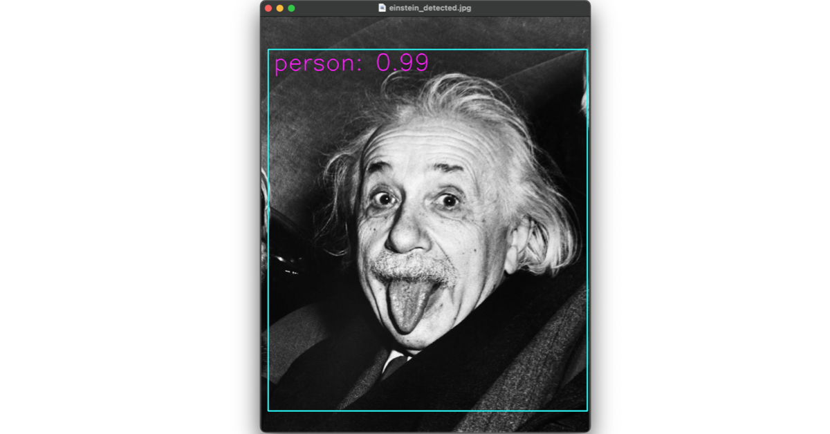
3. 実行 & 結果

python face_detection.py

■ ニューラルネットを使った物体検出

★ Single Shot MultiBox Detector (SSD)

入力画像を一度だけ見て物体認識をする。スピーディーな判読が得意。開発者はWei Liu (2015年)。

• 【論文】SSD: Single Shot MultiBox Detector
• 【web記事】Understand Single Shot MultiBox Detector (SSD) and Implement It in Pytorch

特徴抽出にMultiBoxを使い、物体のスケーリングには入力画像のリサイズで対応する。

実装例 (PyTorch)

PyTorchを使って実装する。²
ソースコードはqfgaohao/pytorch-ssdから拝借。このソースコードは、モデルのベースにMobileNetを使う(本家はVGGがベース)。

1. セットアップ

setup.sh

git clone https://github.com/qfgaohao/pytorch-ssd
wget -P pytorch-ssd/models https://storage.googleapis.com/models-hao/mobilenet-v1-ssd-mp-0_675.pth
wget -P pytorch-ssd/models https://storage.googleapis.com/models-hao/voc-model-labels.txt

2. 実行 & 結果

python run_ssd_live_demo.py mb1-ssd models/mobilenet-v1-ssd-mp-0_675.pth models/voc-model-labels.txt 

デバグ(おまけ)

2のデモでerrorが出た場合の対応例を紹介する。
● カメラのID変更

open VIDEOIO(AVFOUNDATION): raised unknown C++ exception!

のerrorに対して、以下のようにファイルを書き換え。

python;run_ssd_live_demo.py@line21

#cap = cv2.VideoCapture(0) before
cap = cv2.VideoCapture(1) #after

● データタイプの変更(Tensor → Int)

cv2.rectangle(orig_image, (box[0], box[1]), (box[2], box[3]), (255, 255, 0), 4)
TypeError: function takes exactly 4 arguments (2 given)

のerrorに対して、以下のようにファイルを書き換え。

python;run_ssd_live_demo.py@line77&line80

# cv2.rectangle(orig_image, (box[0], box[1]), (box[2], box[3]), (255, 255, 0), 4) before
cv2.rectangle(orig_image, (int(box[0]), int(box[1])), (int(box[2]), int(box[3])), (255, 255, 0), 4) # after
~~
# (box[0]+20, box[1]+40), before
(int(box[0])+20), int(box[1])+40), # after

■ 画像生成

★ Generative Adversarial Networks (GANs, 敵対的生成ネットワーク)

コンピューターも創造的になれることを示したブレイクスルー的なアルゴリスム。多数の学習画像から、新しい画像を生成させることができる。Ian Goodfellowによって開発された(2014年)。

• 【論文】Generative Adversarial Nets
• 【web記事】How do GANs intuitively work?

実装例 (PyTorch)

PyTorchを使って実装する。ソースコードはDeep Learning and Computer Vision A-Z™の他に、DCGAN Tutorialも参考にする。学習に使うデータはチュートリアルのようにCIFAR10やCelebAを使うか、自分で用意する。³

1. セットアップ

touch gans.py
mkdir data results

ディレクトリの構造は以下の通り。

tree
your_working_directory/
├── gans.py
├── data
│   ├── 1.png
│   ...
│   └── 2999.png
└── results

2. メインコード

gans.py

import torch
import torch.nn as nn
import torch.nn.parallel
import torch.optim as optim
import torch.utils.data
import torchvision.datasets as dset
import torchvision.utils as vutils
import torchvision.transforms as transforms
from torch.autograd import Variable
import numpy as np
import matplotlib.pyplot as plt


dataroot = './data/'
batch_size = 64
image_size = 64
num_workers = 0
num_epochs = 100
lr = 0.0002
beta1 = 0.5
nz = 100  # size of generator input
device = torch.device('cuda:0' if (
    torch.cuda.is_available() and ngpu > 0) else 'cpu')
transform = transforms.Compose(
    [transforms.Resize(image_size), transforms.ToTensor()])


dataset = dset.ImageFolder(root=dataroot,
                           transform=transforms.Compose([
                               #                               transforms.Resize(image_size),
                               #                               transforms.CenterCrop(image_size),
                               transforms.ToTensor(),
                               transforms.Normalize(
                                   (0.5, 0.5, 0.5), (0.5, 0.5, 0.5)),
                           ]))
dataloader = torch.utils.data.DataLoader(
    dataset, batch_size=batch_size, shuffle=True, num_workers=num_workers)


def visialize_example(batch):
    plt.figure(figsize=(8, 8))
    plt.axis('off')
    plt.title('training images')
    plt.imshow(np.transpose(vutils.make_grid(batch[0].to(device)[
               :64], padding=2, normalize=True).cpu(), (1, 2, 0)))
    plt.show()


def weights_init(m):
    classname = m.__class__.__name__
    if classname.find('Conv') != -1:
        m.weight.data.normal_(0.0, 0.02)
    elif classname.find('BatchNorm') != -1:
        m.weight.data.normal_(1.0, 0.02)
        m.bias.data.fill_(0)


class G(nn.Module):

    def __init__(self):
        super(G, self).__init__()
        self.main = nn.Sequential(
            nn.ConvTranspose2d(nz, 512, 4, 1, 0, bias=False),
            nn.BatchNorm2d(512),
            nn.ReLU(True),
            nn.ConvTranspose2d(512, 256, 4, 2, 1, bias=False),
            nn.BatchNorm2d(256),
            nn.ReLU(True),
            nn.ConvTranspose2d(256, 128, 4, 2, 1, bias=False),
            nn.BatchNorm2d(128),
            nn.ReLU(True),
            nn.ConvTranspose2d(128, 64, 4, 2, 1, bias=False),
            nn.BatchNorm2d(64),
            nn.ReLU(True),
            nn.ConvTranspose2d(64, 3, 4, 2, 1, bias=False),
            nn.Tanh()
        )

    def forward(self, input):
        output = self.main(input)
        return output


netG = G()
netG.apply(weights_init)


class D(nn.Module):

    def __init__(self):
        super(D, self).__init__()
        self.main = nn.Sequential(
            nn.Conv2d(3, 64, 4, 2, 1, bias=False),
            nn.LeakyReLU(0.2, inplace=True),
            nn.Conv2d(64, 128, 4, 2, 1, bias=False),
            nn.BatchNorm2d(128),
            nn.LeakyReLU(0.2, inplace=True),
            nn.Conv2d(128, 256, 4, 2, 1, bias=False),
            nn.BatchNorm2d(256),
            nn.LeakyReLU(0.2, inplace=True),
            nn.Conv2d(256, 512, 4, 2, 1, bias=False),
            nn.BatchNorm2d(512),
            nn.LeakyReLU(0.2, inplace=True),
            nn.Conv2d(512, 1, 4, 1, 0, bias=False),
            nn.Sigmoid()
        )

    def forward(self, input):
        return self.main(input)
        #output = self.main(input)
        # return output.view(-1)


netD = D()
netD.apply(weights_init)

criterion = nn.BCELoss()
real_label = 1
fake_label = 0
optimizerD = optim.Adam(netD.parameters(), lr=lr, betas=(beta1, 0.999))
optimizerG = optim.Adam(netG.parameters(), lr=lr, betas=(beta1, 0.999))

for epoch in range(num_epochs):
    for i, data in enumerate(dataloader, 0):
        netD.zero_grad()
        real_cpu = data[0].to(device)
        b_size = real_cpu.size(0)
        label = torch.full((b_size,), real_label,
                           dtype=torch.float, device=device)
        output = netD(real_cpu).view(-1)
        errD_real = criterion(output, label)
        errD_real.backward()
        D_x = output.mean().item()

        noise = torch.randn(b_size, nz, 1, 1, device=device)
        fake = netG(noise)
        label.fill_(fake_label)
        output = netD(fake.detach()).view(-1)
        errD_fake = criterion(output, label)
        errD_fake.backward()
        D_G_z1 = output.mean().item()
        errD = errD_real + errD_fake
        optimizerD.step()

        netG.zero_grad()
        label.fill_(real_label)
        output = netD(fake).view(-1)
        errG = criterion(output, label)
        errG.backward()
        D_G_z2 = output.mean().item()
        optimizerG.step()

        if i % 100 == 0:
            print(
                f'[{epoch}/{num_epochs}][{i}/{len(dataloader)}] Loss_D: {errD.data.item()}, Loss_G: {errG.data.item()}')
            vutils.save_image(
                real_cpu, './results/real_samples.png', normalize=True)
            fake = netG(noise)
            vutils.save_image(
                fake, f'./results/fake_samples_epoch_{epoch}.png', normalize=True)

3. 実行 & 結果

python gans.py

■ まとめ

• コンピュータービジョンを学び直し、その内容についてまとめた。

最近これ勉強し直した。
COMPUTER VISION A-Z(TM) IS NOW LIVE! https://t.co/32la5JgjGZ via @YouTube

— honyurui (@isHonyurui) January 29, 2021

---

1. 実行環境: python3.9, opencv4.5, pytorch1.7, GPUなし(Macbook pro, macOS Big Sur) ↩

2. Deep Learning and Computer Vision A-Z™で紹介されている実装がちょっとOutdatedで複雑に感じたので、後日簡単に実装できるものを探した。 ↩

3. 今回の例で使用したEinsteinの顔画像は、Google画像検索から自力で20枚ほど拾ってきた。学習データとして20枚では少ないので、それをImageMagickを使って3000枚に増やし、"data"フォルダに格納した。 ↩