はじめに
TensorFlow 2.0 と Sequence to Sequence の学習のため Translation with Attention チュートリアルに取り組んだ記録として日本語訳や理解したことを残しておきます。
実行環境は Google Colabratory ですが、2.0 Beta 用の Notebook(.ipynb) が見つからなかったため GitHub の少し古い nmt_with_attention.ipynb をベースにコードを差し替えながら進めました。古い方が自力で実装している部分が多いので、その辺りにも触れます。
編集した Notebook は GitHub にコミットしてあります。通常(2.0 Beta)版、各計算段階の形状確認print文を多数入れた版、1.14 ベース版、の 3つありですが、後ろ 2つはおまけです。
この記事を書いてる途中で 2.0 の Notebook を見つけたので取り込みました。また TECH PLAY Magagine さんの日本語訳記事が公開されていました。
Notebook ウォークスルー
ではNotebook を1つ1つ見ていきます。
ただ見ていても頭に入ってきづらい体質なため 1つ 1つ見ながら for ループを内包表記に変えたり、中途半端に型アノテーションを入れたり、80文字以内に収まるよう改行したり、f-string に置き換えたり余計なことをしていますが気にしないでください。
ここでは日本語訳のみ載せています。Attention は訳さずそのまま、など私の好みや不統一な部分はご容赦ください。Notebook には英語と日本語訳どちらも記載しています。
Neural Machine Translation with Attention
このノートブックは tf.keras と eager exicution を使用してスペイン語を英語に翻訳するシーケンス to シーケンス(seq2seq)モデルを学習します。これはシーケンス to シーケンスモデルに関する知識を前提とした高度な例です。
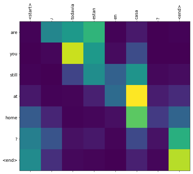
このノートブックでモデルを訓練した後は "¿todavia estan en casa?" などのスペイン語の文章を入力して、英語の翻訳 "are you still at home?" を返すことができます。
翻訳の質は例題としては妥当ですが、生成された Attention プロットはおそらくもっと興味深いものです。これは翻訳中に入力文のどの部分にモデルが注目したかを示します。
注:この例では1台のP100 GPUで実行するのに約10分かかります。
from __future__ import absolute_import
from __future__ import division
from __future__ import print_function
from __future__ import unicode_literals

# Import TensorFlow >= 1.10 and enable eager execution
!pip install tensorflow-gpu==2.0.0-beta1
import tensorflow as tf
# tf.enable_eager_execution()

import matplotlib.pyplot as plt
from sklearn.model_selection import train_test_split

import unicodedata
import re
import numpy as np
import os
import io
import time

print(tf.__version__)
上記のコメント行は元の Notebook が少し古いためで、2.0 のチュートリアルからは削除されています。TensorFrow 2.0 からは eager execution がデフォルトになりますので、tf.enabel_eager_execution()を呼ぶ必要がなくなりました(関数もなくなりました)。
Download and prepare the dataset
データセットのダウンロードと準備(折りたたみ)
- 各文に開始トークンと終了トークンを追加します。
- 特殊文字を削除して文章をきれいにします。
- 単語インデクスと逆単語インデクスを作成します(単語→id と id→単語 のマッピング辞書)。
- 各文を最大長まで埋めます。
# Download the file
path_to_zip = tf.keras.utils.get_file(
    'spa-eng.zip',
    origin='http://storage.googleapis.com/download.tensorflow.org'
        '/data/spa-eng.zip',
    extract=True)

path_to_file = os.path.dirname(path_to_zip) + '/spa-eng/spa.txt'
対訳データファイルをダウンロード&解凍してそのパスを保持しておきます。
# Converts the unicode file to ascii
def unicode_to_ascii(s: str) -> str:
    return ''.join(
        c for c in unicodedata.normalize('NFD', s)
        if unicodedata.category(c) != 'Mn')
UNICODE文字列を正規化し、汎用カテゴリ「Nonspacing_Mark」の文字を除いて返却します。
def preprocess_sentence(w: str) -> str:
    w = unicode_to_ascii(w.lower().strip())

    # creating a space between a word and the punctuation following it
    # eg: "he is a boy." => "he is a boy ."
    # Reference:- https://stackoverflow.com/questions/3645931
    #     /python-padding-punctuation-with-white-spaces-keeping-punctuation
    w = re.sub(r"([?.!,¿])", r" \1 ", w)
    w = re.sub(r'[" "]+', " ", w)

    # replacing everything with space except (a-z, A-Z, ".", "?", "!", ",")
    w = re.sub(r"[^a-zA-Z?.!,¿]+", " ", w)

    w = w.rstrip().strip()

    # adding a start and an end token to the sentence
    # so that the model know when to start and stop predicting.
    w = '<start> ' + w + ' <end>'
    return w
記号の前後に空白を入れ、不要な文字は消して、開始トークン <start> と終了トークン <end> を付けて返却します。
細かいですが、スペイン語の文頭の「¿」(逆ハテナ)は残すのに、「¡」(逆ビックリ)は残さない理由が不明でした。3つ目の re.sub() に対するコメントは (a-z, A-Z, ".", "?", "!", ",") を除いて空白に置換する、となっていて「¿」は空白に置換される対象に読めますが、コード上は「¿」も除外されています。あってもなくても翻訳精度には影響しなそうなのですが、少し気になりました。
en_sentence = 'May I borrow this book?'
sp_sentence = '¿Puedo tomar prestado este libro?'
print(preprocess_sentence(en_sentence))
print(preprocess_sentence(sp_sentence).encode('utf-8'))
<start> may i borrow this book ? <end>
b'<start> \xc2\xbf puedo tomar prestado este libro ? <end>'
preprocess_sentence() の動作確認です。
# 1. Remove the accents
# 2. Clean the sentences
# 3. Return word pairs in the format: zip[ENGLISH(Tuple), SPANISH(Tuple)]
def create_dataset(path: str, num_examples: int) -> zip:
    lines = open(path, encoding='UTF-8').read().strip().split('\n')

    word_pairs = [
        [preprocess_sentence(w) for w in l.split('\t')]
        for l in lines[:num_examples]
    ]

    return zip(*word_pairs)
対訳データは英語とスペイン語がタブで区切られていて、タブで分割したそれぞれに preprocess_sentence() を実行して返却しています。以前の Notebook では word_pairs をそのまま返却していたので index 0 が英語、1 がスペイン語である要素数 2 のリストを対訳ペア数分持ったリストが返却されていました。
その形式だと内包表記を使って英語だけ抽出、スペイン語だけ抽出、とする必要があって少しだけ面倒でしたが、2.0 Beta では word_pairs を展開したものを zip しており、1 回目に英語すべての Tuple、2 回目にスペイン語すべての Tuple が列挙される zip オブジェクトが返却されるようになり少し処理しやすくなっています。冒頭のコメント # 3. を書き換えてみましたが表現が微妙です。
ちなみに zip オブジェクトの中身まで示す型アノテーションってどう書くんでしょうか。Iterable[str] とかしか思いつきませんでした。
en, sp = create_dataset(path_to_file, None)
print(en[-1])
print(sp[-1])
<start> if you want to sound like a native speaker , you must be willing to practice saying the same sentence over and over in the same way that banjo players practice the same phrase over and over until they can play it correctly and at the desired tempo . <end>
<start> si quieres sonar como un hablante nativo , debes estar dispuesto a practicar diciendo la misma frase una y otra vez de la misma manera en que un musico de banjo practica el mismo fraseo una y otra vez hasta que lo puedan tocar correctamente y en el tiempo esperado . <end>
create_dataset() の動作確認です。
以前の Notebook にはなかったセルで、地味にやさしくなっているようです。
def max_length(tensor):
    return max(len(t) for t in tensor)
リストの中の要素の最大長を求めます。あとで訓練データの入力シーケンス最大長や、正解データの最大長を求めるのに使います。
def tokenize(
    lang: Sequence[str]
) -> Tuple[np.ndarray, tf.keras.preprocessing.text.Tokenizer]:

    lang_tokenizer = tf.keras.preprocessing.text.Tokenizer(filters='')
    lang_tokenizer.fit_on_texts(lang)

    tensor = lang_tokenizer.texts_to_sequences(lang)
    tensor = tf.keras.preprocessing.sequence.pad_sequences(
        tensor,
        padding='post')

    return tensor, lang_tokenizer
Tokenizer と pad_sequences を使って空白区切りの文字列シーケンスを単語インデクスの整数シーケンスに変換(Tokenize)し、変換後のシーケンスと Tokenizer オブジェクトを返却します。
以前の Notebook では tokenize() 関数はなく、word to index と index to word 辞書を作成する LanguageIndex クラスの実装があり、この次に出てくる load_dataset() 関数内で word to index 辞書と pad_sequences() による整数シーケンスへの変換を行っていました。以前の Notebook の方が tokenize の実態のイメージを掴めるかも知れません。
def load_dataset(path: str, num_examples: int = None):
    # creating cleaned input, output pairs
    targ_lang, inp_lang = create_dataset(path, num_examples)

    input_tensor, inp_lang_tokenizer = tokenize(inp_lang)
    target_tensor, targ_lang_tokenizer = tokenize(targ_lang)

    return input_tensor, target_tensor, inp_lang_tokenizer, targ_lang_tokenizer
これまでに定義した関数を使って対訳データファイルからデータセットを読み込みます。
引数 num_examples はファイルの何行目までを返却するか制御しますが、2.0 Beta から既定値が None になり、意図的に None を指定しなくてもファイルパスだけ指定すれば全件返却されるようになりました。
Limit the size of the dataset to experiment faster (optional)
10万文を超える完全なデータセットのトレーニングには長い時間がかかります。より早く訓練するために、データセットのサイズを3万文に制限することができます(もちろん少ないデータでは翻訳品質が低下します)。
# Try experimenting with the size of that dataset
num_examples = None  # 30000
input_tensor, target_tensor, inp_lang, targ_lang = load_dataset(
    path_to_file,
    num_examples)

# Calculate max_length of the input tensors and the target tensors
max_length_inp = max_length(input_tensor)
max_length_targ = max_length(target_tensor)
# Creating training and validation sets using an 80-20 split
(input_tensor_train, input_tensor_val,
 target_tensor_train, target_tensor_val) = train_test_split(
    input_tensor,
    target_tensor,
    test_size=0.2)

# Show length
(len(input_tensor_train), len(target_tensor_train),
 len(input_tensor_val), len(target_tensor_val))
load_dateset() でファイルから対訳データを読み出し、入力データと翻訳データを8:2の割合で訓練用と検証用に分けます。load_dataset() の num_expamles は元々 30000 を指定していましたが、全データ処理するためここでは None を指定しています。
30000 件だと 1 epoch 50秒程度ですが、全件(118964件)だと 1 epoch 18 分ほど掛かりました。
def convert(lang, tensor):
    for t in tensor:
        if t != 0:
            print("%d ----> %s" % (t, lang.index_word[t]))
print("Input Language; index to word mapping")
convert(inp_lang, input_tensor_train[0])
print()
print("Target Language; index to word mapping")
convert(targ_lang, target_tensor_train[0])
Input Language; index to word mapping
1 ----> <start>
2188 ----> ponte
6 ----> el
682 ----> sombrero
3 ----> .
2 ----> <end>

Target Language; index to word mapping
1 ----> <start>
175 ----> put
35 ----> your
698 ----> hat
36 ----> on
3 ----> .
2 ----> <end>
トークナイザーの index_word 辞書による変換イメージ確認です。
Create a tf.data dataset
BUFFER_SIZE = len(input_tensor_train)
BATCH_SIZE = 64
steps_per_epoch = BUFFER_SIZE // BATCH_SIZE
embedding_dim = 256
units = 1024
vocab_inp_size = len(inp_lang.word_index) + 1
vocab_tar_size = len(targ_lang.word_index) + 1

dataset = tf.data.Dataset.from_tensor_slices(
    (input_tensor_train, target_tensor_train)).shuffle(BUFFER_SIZE)
dataset = dataset.batch(BATCH_SIZE, drop_remainder=True)
各種ハイパーパラメーターを定義し、データをシャッフルした上で連続データをまとめてバッチ化します。
バッチのイメージ確認として 1つ目のバッチを取り出して形状を表示します。スペイン語は最大 53 トークン、英語は最大 51 トークンになっています。
example_input_batch, example_target_batch = next(iter(dataset))
example_input_batch.shape, example_target_batch.shape
(TensorShape([64, 53]), TensorShape([64, 51]))
エンコーダーとデコーダーモデルの記述(折りたたみ)
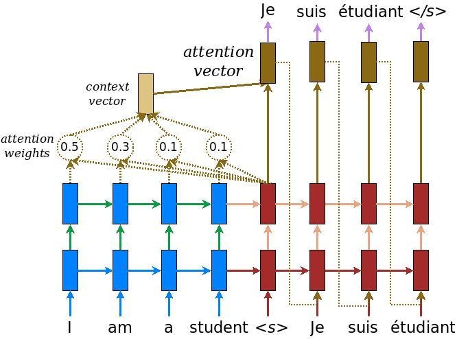
入力はエンコーダーモデルを通過します。これにより形状が (batch_size, max_length, hidden_size) のエンコーダー出力と、形状が (batch_size, hidden_size) のエンコーダー隠れ状態が得られます。
これが実装される計算式です:
私たちは Bahdanau attention を使います。簡略形で書く前に表記法を決めましょう。
- FC = Fully connected (dense) layer:全結合層
- EO = Encoder output:エンコーダー出力
- H = hidden state:隠れ状態
- X = input to the decoder:デコーダー入力
そして擬似コードです。
-
score = FC(tanh(FC(EO) + FC(H)))
メモ:全結合層は入力と内部の重みの行列積を計算するレイヤーのため、計算式中で $W_1$ や $v_a$ などの重みとの積の部分はFCにより表現できる。ここで $h_t$ =H、$\bar{h}_s$ =EO。 -
attention weights = softmax(score, axis = 1)
Softmax はデフォルトでは最後の軸に適用されますが、ここではスコアの形状が (batch_size, max_length, 1) であるため、1番目の軸 に適用します。Max_lengthは私達の入力の長さです。各入力に重みを割り当てようとしているので softmax をその軸に適用する必要があります。 -
context vector = sum(attention weights * EO, axis = 1)
1番目の軸を選択したのは上と同じ理由です。 -
embedding output= デコーダーへの入力 X は埋め込み層を通過する。 merged vector = concat(embedding output, context vector)- このマージされたベクトルは GRU に渡されます
各ステップのすべてのベクトルの形状はコード内のコメントで指定されています。
class Encoder(tf.keras.Model):
    def __init__(
            self,
            vocab_size: int,  # 語彙数
            embedding_dim: int,  # 埋め込みレイヤーで出力する密ベクトルの次元数
            enc_units: int,  # Encoder(のGRU)の出力次元数
            batch_sz: int):  # バッチサイズ

        super(Encoder, self).__init__()
        self.batch_sz = batch_sz
        self.enc_units = enc_units
        self.embedding = tf.keras.layers.Embedding(vocab_size, embedding_dim)
        self.gru = tf.keras.layers.GRU(
            self.enc_units,
            return_sequences=True,
            return_state=True,
            recurrent_initializer='glorot_uniform')

    # 入力 x は int の ndarray を convert_to_tensor() したもの
    # 型としては tensorflow.python.framework.ops.EagerTensor …
    # hidden は初回は initialze_hidden_state で返却したものが渡ってくる
    def call(self, x, hidden):
        x = self.embedding(x)
        output, state = self.gru(x, initial_state=hidden)
        return output, state

    def initialize_hidden_state(self):
        return tf.zeros((self.batch_sz, self.enc_units))
まずはエンコーダーの実装です。keras でカスタムモデルを作成する場合、Model クラスを継承して __init__() でパラメーターの保存やレイヤーの作成を、call() で順伝播処理を実装します。エンコーダーで必要なのは入力である単語インデクスの整数シーケンスを密ベクトル化する Embedding レイヤーと、それを再帰的に学習、処理する GRU レイヤーだけのため実装量は少ないです。
2.0 Beta 以前では CuDNNGRU レイヤーと GRU レイヤーにクラスが分かれていて、tf.test.is_gpu_available() により GPU が利用可能かどうかを判定して生成するクラスを分岐していましたが、GRU レイヤークラスに 1本化され GPU 利用条件を満たす場合は自動的に GPU を利用するようになりました。GPU 利用条件はこの下の抜粋訳を参照してください。
Embedding
メモ:Embedding レイヤーは入力の整数値(単語ID)を固定長の密ベクトルに変換します。第 1引数 input_dim は語彙数。第2引数 output_dim は出力する密ベクトルの次元数。
GRU
※GPUが使われる条件について抜粋※
利用可能なランタイムハードウェアと制約に基づいて、このレイヤーはパフォーマンス最大化のため異なる実装(cuDNN ベースまたは純粋なTensorFlow)を選択します。 GPU が利用可能で、レイヤーに対するすべての引数が CuDNN カーネルの要件を満たす場合(詳細は下記を参照)、高速な cuDNN 実装を使用します。
cuDNN 実装を使用するための要件は次のとおりです。
- activation == 'tanh'
- recurrent_activation == 'sigmoid'
- recurrent_dropout == 0
- unroll is False
- use_bias is True
- reset_after is True
- 入力がマスクされていないか、厳密に右詰めされている
メモ:1 ~ 6 は既定値のため、この入力値の条件さえ満たせば GPU が使われます
encoder = Encoder(vocab_inp_size, embedding_dim, units, BATCH_SIZE)

# sample input
sample_hidden = encoder.initialize_hidden_state()
sample_output, sample_hidden = encoder(example_input_batch, sample_hidden)
print('Encoder output shape: (batch size, sequence length, units) '
      f'{sample_output.shape}')
print('Encoder Hidden state shape: (batch size, units) '
      f'{sample_hidden.shape}')
Encoder output shape: (batch size, sequence length, units) (64, 53, 1024)
Encoder Hidden state shape: (batch size, units) (64, 1024)
エンコーダーモデルの生成と、エンコーダー出力および隠れ状態の形状表示。各計算段階でのデータ形状は以下のとおりです。
| 計算段階 | 形状 | 備考 |
|---|---|---|
| 入力 | (batch_sz, max_length_inp) = (64, 53) | |
| Embedding後 | (batch_sz, max_length_inp, embedding_dim) = (64, 53, 256) | 1単語が 256次元の密ベクトルになる |
| 出力 | (batch_sz, max_length_inp, units) = (64, 53, 1024)) | GRU レイヤーの出力次元は指定したユニット数 |
| 隠れ状態 | (batch_sz, units) = (64, 1024) | 単語を全て処理した後の隠れ状態のため 1×ユニット数の形状になる |
| GRU では出力と隠れ状態が等しいため、上記出力の max_length_inp 軸末尾の出力値と、隠れ状態の値は同じ値です。 |
class BahdanauAttention(tf.keras.Model):
    def __init__(self, units):
        super(BahdanauAttention, self).__init__()
        self.W1 = tf.keras.layers.Dense(units)
        self.W2 = tf.keras.layers.Dense(units)
        self.V = tf.keras.layers.Dense(1)

    def call(self, query, values):
        # hidden shape == (batch_size, hidden size)
        # hidden_with_time_axis shape == (batch_size, 1, hidden size)
        # we are doing this to perform addition to calculate the score
        hidden_with_time_axis = tf.expand_dims(query, 1)

        # score shape == (batch_size, max_length, 1)
        # we get 1 at the last axis because we are applying score to self.V
        # the shape of the tensor before applying self.V is
        # (batch_size, max_length, units)
        score = self.V(tf.nn.tanh(
            self.W1(values) + self.W2(hidden_with_time_axis)))

        # attention_weights shape == (batch_size, max_length, 1)
        attention_weights = tf.nn.softmax(score, axis=1)

        # context_vector shape after sum == (batch_size, hidden_size)
        context_vector = attention_weights * values
        context_vector = tf.reduce_sum(context_vector, axis=1)

        return context_vector, attention_weights
Bahdanau アテンション(のコンテキストベクトル)を計算するカスタムモデルを定義しています。
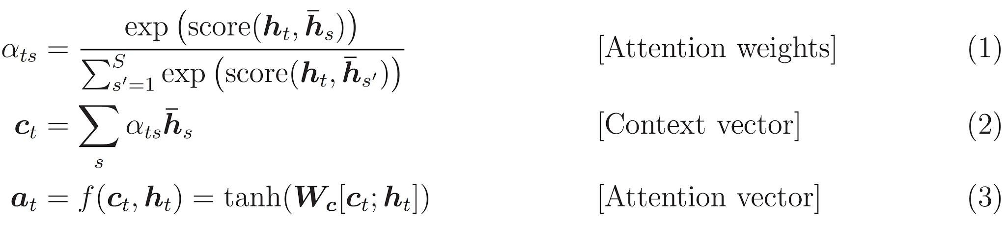
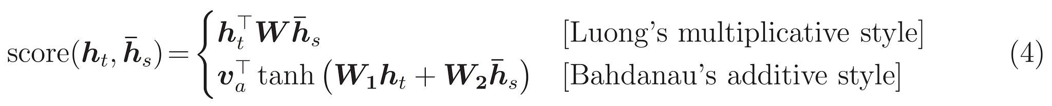
以前の Notebook ではこの次に出てくる Decoder クラス内にすべて実装されていましたが、独立したことで分かりやすくなりました。このクラス内で実装する計算式を再掲します。
\begin{align}
score(h_t, \bar{h}_s) & = v^T_a tanh (W_1 h_t + W_2 \bar{h}_s) \tag{4} \\\\
\alpha_{ts} & = \frac{\exp(score(h_t, \bar{h}_s))}{\sum^S_{s'=1}\exp(score(h_t, \bar{h}_{s'}))} \tag{1} \\\\
c_t & = \sum_s \alpha_{ts} \bar{h}_s \tag{2}
\end{align}
まず $(4)$ の $score$ の計算ですが、$h_t$はデコーダー隠れ状態(query)、$\bar{h}_s$はエンコーダー出力(values)です。重み $v^T_a$、$W_1$、$W_2$ との積は全結合層を通すことで表現します。隠れ状態やエンコーダー出力のトークンごとの次元は units(=1024) ですが、$score$ は 1つの実数値(=1)のため、$v^T_a$ の全結合層の出力次元は 1 になっています。
エンコーダー出力の形状が (batch_sz, max_length_inp, units)、隠れ状態の形状が (batch_sz, units) で階層が合っていないため tf.expand_dims(axis=1) により階層を合わせて足し算(ブロードキャスト)を行います。
余談ですが、計算式では$W_1$ に $h_t$(=query)、$W_2$ に $\bar{h}_s$(=values) を掛けていますが、コード上では逆の組み合わせになっていて非常に紛らわしかったです。
$(1)$ のアテンション重み $\alpha_{ts}$ はトークン(max_length_inpの軸)に対する softmax を表しているので、tf.nn.softmax(axis=1) で求まります。
$(2)$ のコンテキストベクトル $c_t$ も $\alpha_{ts}$ と $\bar{h}_s$ の要素同士の積を求め、全トークン分(max_length_inpの軸)加算して求めます。コンテキストベクトルを求めた以降、訓練でも翻訳でもアテンション重みは使いませんが、戻り値として返しているのはプロットするためです。
各計算段階でのデータ形状は以下のとおりです。
| 計算段階 | 形状 | 備考 |
|---|---|---|
| エンコーダー出力 $\bar{h}_s$ | (batch_sz, max_length_inp, units) = (64, 53, 1024) | 引数 values |
| デコーダー隠れ状態 $h_t$ | (batch_sz, units) = (64, 1024) | 引数 query |
| 隠れ状態軸追加 | (batch_sz, 1, units) = (64, 1, 1024) | hidden_with_time_axis |
| $\tanh(W_1 h_t + W_2 \bar{h}_s)$ | (batch_sz, max_length_inp, units) = (64, 53, 1024) | |
| $score$ | (batch_sz, max_length_inp, 1)=(64, 53, 1) | $v^T_a$ の出力次元 = 1 |
| アテンション重み $\alpha_{ts}$ | (batch_sz, max_length_inp, 1) = (64, 53, 1) | attention_weights |
| コンテキストベクトル $c_t$ | (batch_sz, units) = (64, 1024) | context_vector |
class Decoder(tf.keras.Model):
    def __init__(
        self,
        vocab_size: int,  # 語彙数
        embedding_dim: int,  # 埋め込みレイヤーで出力する密ベクトルの次元数
        dec_units: int,  # GRU の出力次元数
        batch_sz: int):  # バッチサイズ

        super(Decoder, self).__init__()
        self.batch_sz = batch_sz
        self.dec_units = dec_units
        self.embedding = tf.keras.layers.Embedding(vocab_size, embedding_dim)
        self.gru = tf.keras.layers.GRU(
            self.dec_units,
            return_sequences=True,  # 入力の全単語分の出力を返す
            return_state=True,  # 隠れ状態を返す
            recurrent_initializer='glorot_uniform')
        self.fc = tf.keras.layers.Dense(vocab_size)

        # used for attention
        self.attention = BahdanauAttention(self.dec_units)

    def call(self, x, hidden, enc_output):
        # enc_output shape == (batch_size, max_length, hidden_size)
        context_vector, attention_weights = self.attention(hidden, enc_output)

        # x shape after passing through embedding ==
        # (batch_size, 1, embedding_dim)
        x = self.embedding(x)

        # x shape after concatenation ==
        # (batch_size, 1, embedding_dim + hidden_size)
        x = tf.concat([tf.expand_dims(context_vector, 1), x], axis=-1)

        # passing the concatenated vector to the GRU
        output, state = self.gru(x)

        # output shape == (batch_size * 1, hidden_size)
        output = tf.reshape(output, (-1, output.shape[2]))

        # output shape == (batch_size, vocab)
        x = self.fc(output)

        return x, state, attention_weights
つづいてデコーダーの実装です。デコーダーも、まず入力の単語インデクス整数値を固定長密ベクトルに変換する Embedding レイヤーを通します。次が GRU レイヤーである点も一緒ですが、Enbedding したベクトルではなく(まだ実装していない)次式のアテンションベクトルを渡します。
a_t = f(c_t, h_t) = \tanh(W_c [C_t; h_t]) \tag{3} \\
と、そんな風に考えていた時期が俺にもありました。
call メソッドには x = tf.concat([tf.expand_dims(context_vector, 1), x], axis = -1) とあり、これが $[C_t; h_t]$ に対応するような気がしていたが別にそんなことはなかったぜ。x は入力の単語ベクトルであって隠れ状態 $h_t$ ではないですし、$W_c$ や $\tanh$ に対応するコードもありません。見たまんま、コンテキストベクトルと単語ベクトルを結合したベクトルを GRU に渡しています。ただ、この 2つを concat したベクトルを渡せば良い、という他の情報が見つかりませんでした。原論文を(読まずに)ざっと見ても無さそうでしたし、こちらの記事ではコンテキストベクトルと「時刻t-1 の隠れ状態」を concat すると書いてありました。
疑問は残りますが上の方で擬似コードとして書かれていた以下の記述に則したコードではあるので深追いしないことにします。
-
embedding output= デコーダーへの入力 X は埋め込み層を通過する。 merged vector = concat(embedding output, context vector)- このマージされたベクトルは GRU に渡されます
GRU を通したあとの出力を reshape していますが、デコーダーの入力は最初は開始トークン、次は開始トークンに対して予測した単語、…と 1単語ずつ入力されてループする形ですので、GRU 出力の形状は (batch_sz, 1, units) になります。axis = 1 の軸は不要なためこれを reshape によって削減し (batch_sz, units) にしています。
最後に、出力をターゲットの単語に対応付けられるよう、出力次元をターゲット語彙数に指定した全結合層にかけてデコーダーは終了です。
decoder = Decoder(vocab_tar_size, embedding_dim, units, BATCH_SIZE)

sample_decoder_output, _, _ = decoder(
    tf.random.uniform((BATCH_SIZE, 1)),
    sample_hidden,
    sample_output)

print('Decoder output shape: (batch_size, vocab size) '
      f'{sample_decoder_output.shape}')
Decoder output shape: (batch_size, vocab size) (64, 12934)
デコーダーモデルの生成と、デコーダー出力の形状表示。各計算段階でのデータ形状は以下のとおりです。
| 計算段階 | 形状 | 備考 |
|---|---|---|
| デコーダー入力 | (batch_sz, 1) = (64, 1) | x。1単語ずつ |
| Embedding後 | (batch_sz, 1, embedding_dim) = (64, 1, 256) | x |
| コンテキストベクトル $c_t$ | (batch_sz, units) = (64, 1024) | context_vector |
| concat後 | (batch_sz, 1, embedding_dim+units) = (64, 1, 1280) | x |
| GRU 出力 | (batch_sz, 1, units) = (64, 1, 1024) | output |
| reshape後 | (batch_sz, units) = (64, 1024) | x。なぜ x? |
| 全結合後 | (batch_sz, vocab_tar_size) = (64, 12934) | x |
モデルの仕上げとか訓練とかテスト翻訳とか(折りたたみ)
optimizer = tf.keras.optimizers.Adam()
loss_object = tf.keras.losses.SparseCategoricalCrossentropy(
    from_logits=True,
    reduction='none')

def loss_function(real, pred):
    mask = tf.math.logical_not(tf.math.equal(real, 0))
    loss_ = loss_object(real, pred)

    mask = tf.cast(mask, dtype=loss_.dtype)
    loss_ *= mask

    return tf.reduce_mean(loss_)
Checkpoints (Object-based saving)
checkpoint_dir = './training_checkpoints'
checkpoint_prefix = os.path.join(checkpoint_dir, "ckpt")
checkpoint = tf.train.Checkpoint(
    optimizer=optimizer,
    encoder=encoder,
    decoder=decoder)
Training
- 出力と隠れ状態を返すエンコーダーに入力を渡します。
- エンコーダーの出力と隠れ状態、およびデコーダー入力(開始トークン)がデコーダーに渡されます。
- デコーダーは予測結果とデコーダー隠れ状態を返します。
- デコーダー隠れ状態がモデルに戻され、予測結果が損失の計算に使用されます。
- デコーダーへの次の入力を決定するために teacher forcing を使用します。
- Teacher forcing はターゲット(正解)の単語を次の入力としてデコーダーに渡す手法です。
- 最後のステップは勾配を計算し、それをオプティマイザに適用して逆伝播することです。
@tf.function
def train_step(inp, targ, enc_hidden):
    loss = 0

    with tf.GradientTape() as tape:
        enc_output, enc_hidden = encoder(inp, enc_hidden)

        dec_hidden = enc_hidden

        dec_input = tf.expand_dims(
            [targ_lang.word_index['<start>']] * BATCH_SIZE, 1)

        # Teacher forcing - feeding the target as the next input
        for t in range(1, targ.shape[1]):
            # passing enc_output to the decoder
            predictions, dec_hidden, _ = decoder(
                dec_input,
                dec_hidden,
                enc_output)

            loss += loss_function(targ[:, t], predictions)

            # using teacher forcing
            dec_input = tf.expand_dims(targ[:, t], 1)

    batch_loss = (loss / int(targ.shape[1]))

    variables = encoder.trainable_variables + decoder.trainable_variables

    gradients = tape.gradient(loss, variables)

    optimizer.apply_gradients(zip(gradients, variables))

    return batch_loss
補足程度ですが、時刻 t の decoder の戻り値 dec_hidden が for ループの次(時刻 t + 1)の処理で decoder に渡されます。
同様に targ[:, t] が dec_input として次の for ループで渡されますが、これが teacher forcing になります。
EPOCHS = 10

for epoch in range(EPOCHS):
    start = time.time()

    enc_hidden = encoder.initialize_hidden_state()
    total_loss = 0

    for (batch, (inp, targ)) in enumerate(dataset.take(steps_per_epoch)):
        batch_loss = train_step(inp, targ, enc_hidden)
        total_loss += batch_loss

        if batch % 100 == 0:
            print(f'Epoch {epoch + 1} Batch {batch} '
                  f'Loss {batch_loss.numpy():.4f}')

    # saving (checkpoint) the model every 2 epochs
    if (epoch + 1) % 2 == 0:
        checkpoint.save(file_prefix = checkpoint_prefix)

    print(f'Epoch {epoch + 1} Loss {total_loss / steps_per_epoch:.4f}')
    print(f'Time taken for 1 epoch {time.time() - start} sec\n')
Translate
- 評価関数は teacher forcing を使用しないことを除いてトレーニングループと似ています。各時間ステップのデコーダーへの入力は、1つ前の予測値および隠れ状態とエンコーダー出力です。
- モデルが終了トークンを予測したら予測を停止します。
- そしてタイムステップごとに attention weights を保存します。
注:エンコーダー出力は1つの入力に対して1回だけ計算されます。
def evaluate(sentence):

    attention_plot = np.zeros((max_length_targ, max_length_inp))

    sentence = preprocess_sentence(sentence)

    inputs = [inp_lang.word_index[i] for i in sentence.split(' ')]
    inputs = tf.keras.preprocessing.sequence.pad_sequences(
        [inputs],
        maxlen=max_length_inp,
        padding='post')
    inputs = tf.convert_to_tensor(inputs)

    result = ''

    hidden = [tf.zeros((1, units))]
    enc_out, enc_hidden = encoder(inputs, hidden)

    dec_hidden = enc_hidden
    dec_input = tf.expand_dims([targ_lang.word_index['<start>']], 0)

    for t in range(max_length_targ):
        predictions, dec_hidden, attention_weights = decoder(
            dec_input,
            dec_hidden,
            enc_out)

        # storing the attention weights to plot later on
        attention_weights = tf.reshape(attention_weights, (-1,))
        attention_plot[t] = attention_weights.numpy()

        predicted_id = tf.argmax(predictions[0]).numpy()

        result += targ_lang.index_word[predicted_id] + ' '

        if targ_lang.index_word[predicted_id] == '<end>':
            return result, sentence, attention_plot

        # the predicted ID is fed back into the model
        dec_input = tf.expand_dims([predicted_id], 0)

    return result, sentence, attention_plot
評価関数でトレーニング時と違う箇所は、decoder が返した attention_wights を描画用に保持して返却する点と、decoder 出力値の argmax をとってターゲットの単語インデクスに変換しているところです。
# function for plotting the attention weights
def plot_attention(attention, sentence, predicted_sentence):
    fig = plt.figure(figsize=(5, 5))
    ax = fig.add_subplot(1, 1, 1)
    ax.matshow(attention, cmap='viridis')

    fontdict = {'fontsize': 11}

    ax.set_xticklabels([''] + sentence, fontdict=fontdict, rotation=90)
    ax.set_yticklabels([''] + predicted_sentence, fontdict=fontdict)

    plt.show()
アテンション重みのプロットサイズが大きかったので figsize = (5, 5) に変更しています。
def translate(sentence):

    result, sentence, attention_plot = evaluate(sentence)

    print(f'Input: {sentence}')
    print(f'Predicted translation: {result}')

    attention_plot = attention_plot[
        :len(result.split(' ')), :len(sentence.split(' '))]
    plot_attention(attention_plot, sentence.split(' '), result.split(' '))
Restore the latest checkpoint and test
# restoring the latest checkpoint in checkpoint_dir
checkpoint.restore(tf.train.latest_checkpoint(checkpoint_dir))
translate('hace mucho frio aqui.')
Input: <start> hace mucho frio aqui . <end>
Predicted translation: it s very cold here . <end>
translate('esta es mi vida.')
Input: <start> esta es mi vida . <end>
Predicted translation: this is my life . <end>
translate('todavia estan en casa?')
Input: <start> todavia estan en casa ? <end>
Predicted translation: they re still at home . <end>
# wrong translation
translate('trata de averiguarlo.')
Input: <start> trata de averiguarlo . <end>
Predicted translation: try to figure it . <end>
Next steps
- 別のデータセットをダウンロードして、たとえば英語からドイツ語、または英語からフランス語への翻訳を試してください。
- より大きなデータセットでのトレーニング、またはより多くのエポックの使用を試してください。
参考
以下のブログや記事を Attention 理解の参考にさせて頂きました。
- 論文解説 Attention Is All You Need (Transformer)
- よくわかる注意機構(Attention)
- seq2seq で長い文の学習をうまくやるための Attention Mechanism について
おわりに
後半コメントが薄くなってしまいましたが以上です。時間をかけて Notebook を実行して理解を深めたつもりでしたが、この記事を書きながら再度見直したことで更なる気付きが得られました。
一部疑問点が残っていますし、原論文からするとおかしい部分もあるかも知れませんので、教えて頂けると嬉しいです。
この次は記事を書けるかは別として Transformer、BERT を理解していく予定です。