Pythonを用いてデータを補間する方法

データを補間するときのオプションについて，参考となるスクリプトと図を示す

補間方法によっては，元のデータからかけ離れた値となってしまうことに注意

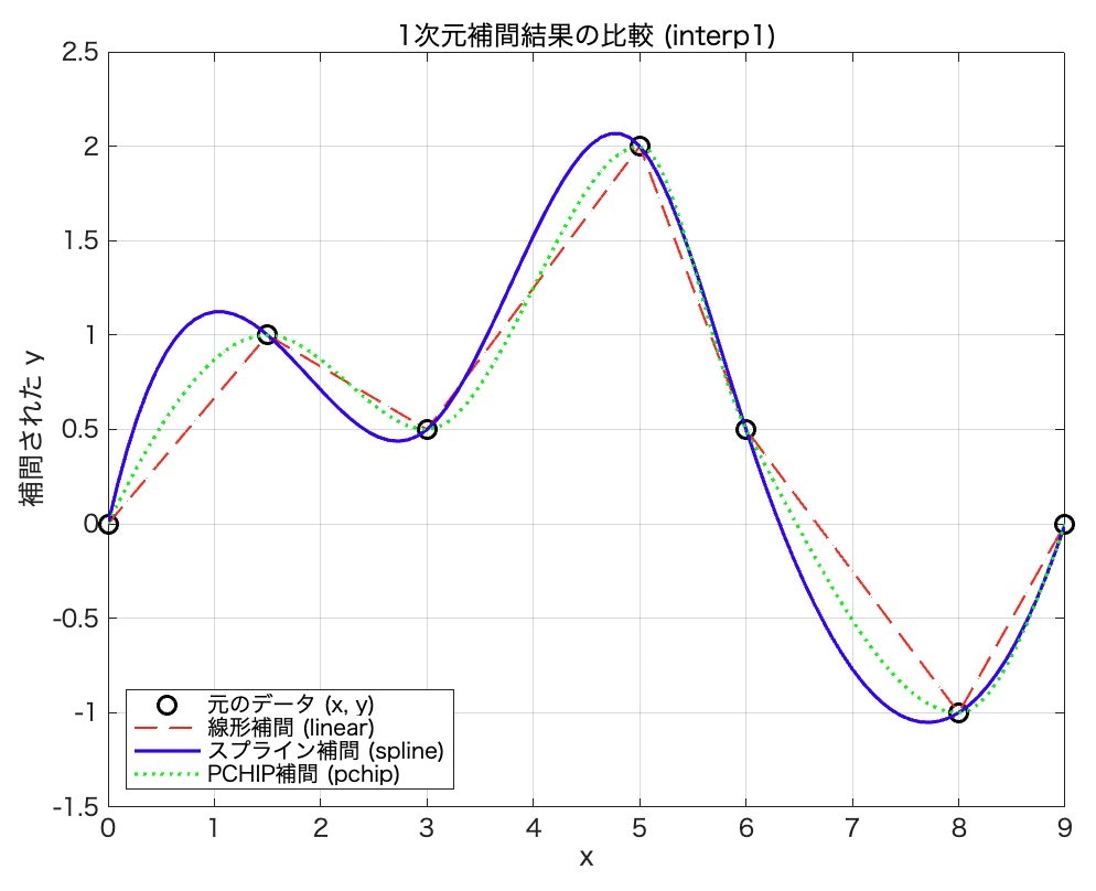
科学データなどを扱う際には，安易にスプライン補間をしてしまうと，滑らかなカーブを生成しようとして，データが急変するところではオーバーシュートしてしまう．

それに対して，pchip（区分的三次エルミート補間多項式）では，元データの単調性を考慮してくれる．

工学的なデータ（物質の密度・温度の上昇・化学反応の濃度変化など，単調性や非負性が崩れてはいけないデータ）の補間時に利用するといい．

my_interp.py

import numpy as np
import matplotlib.pyplot as plt
from scipy.interpolate import interp1d

# 1. 元データ (x, y) の定義
x = np.array([0, 1.5, 3, 5, 6, 8, 9]) # 既知の x 座標
y = np.array([0, 1, 0.5, 2, 0.5, -1, 0]) # 既知の y 座標

# 2. 補間したい点 (xx) の定義 (元のデータよりも密な点)
xx = np.linspace(x.min(), x.max(), 100) # xの範囲内で100点の均等なベクトル

# 3. 異なる補間方法で値を計算
# SciPyの interp1d 関数を使用します。
# 'linear': 線形補間
f_linear = interp1d(x, y, kind='linear')
yy_linear = f_linear(xx)

# 'cubic': 三次スプライン補間 (MATLABの 'spline' に相当)
f_spline = interp1d(x, y, kind='cubic')
yy_spline = f_spline(xx)

# 'pchip': 区分的三次エルミート補間 (MATLABの 'pchip' に相当)
# SciPyでは 'pchip' と指定できます
f_pchip = interp1d(x, y, kind='pchip')
yy_pchip = f_pchip(xx)

# 'nearest': 最近傍点補間 (参考)
# f_nearest = interp1d(x, y, kind='nearest')
# yy_nearest = f_nearest(xx)

# 4. 結果の図示 (プロット)
plt.figure(figsize=(10, 6))

# 元のデータ点をプロット（マーカー 'o' で強調）
plt.plot(x, y, 'ko', markersize=8, label='元のデータ (x, y)')

# 各補間結果をプロット
plt.plot(xx, yy_linear, 'r--', linewidth=1, label='線形補間 (linear)')
plt.plot(xx, yy_spline, 'b-', linewidth=1.5, label='スプライン補間 (cubic)')
plt.plot(xx, yy_pchip, 'g:', linewidth=1.5, label='PCHIP補間 (pchip)')

# グラフの装飾
plt.title('Python (SciPy) における1次元補間結果の比較')
plt.xlabel('x')
plt.ylabel('補間された y')
plt.legend(loc='southwest') 
plt.grid(True)
plt.show() # グラフを表示

参考：MATLABスクリプト

my_interp.m

% 1. 元データ (x, y) の定義
x = [0, 1.5, 3, 5, 6, 8, 9]; % 既知の x 座標
y = [0, 1, 0.5, 2, 0.5, -1, 0]; % 既知の y 座標

% 2. 補間したい点 (xx) の定義 (元のデータよりも密な点)
xx = linspace(min(x), max(x), 100); % xの範囲内で100点の均等なベクトル

% 3. 異なる補間方法で値を計算
% 線形補間 ('linear'): 隣接点を直線で結ぶ
yy_linear = interp1(x, y, xx, 'linear'); 

% スプライン補間 ('spline'): 全体を滑らかな曲線で結ぶ
yy_spline = interp1(x, y, xx, 'spline'); 

% PCHIP補間 ('pchip'): 単調性を保持した三次多項式で結ぶ
yy_pchip = interp1(x, y, xx, 'pchip'); 

% 4. 結果の図示 (プロット)
figure;

% 元のデータ点をプロット（マーカー 'o' で強調）
plot(x, y, 'ko', 'MarkerSize', 8, 'LineWidth', 1.5, 'DisplayName', '元のデータ (x, y)');
hold on; % 続けて他の線を重ねて描画

% 各補間結果をプロット
plot(xx, yy_linear, 'r--', 'LineWidth', 1, 'DisplayName', '線形補間 (linear)');
plot(xx, yy_spline, 'b-', 'LineWidth', 1.5, 'DisplayName', 'スプライン補間 (spline)');
plot(xx, yy_pchip, 'g:', 'LineWidth', 1.5, 'DisplayName', 'PCHIP補間 (pchip)');

% グラフの装飾
title('1次元補間結果の比較 (interp1)');
xlabel('x');
ylabel('補間された y');
legend('Location', 'southwest'); % 凡例を左下に配置
grid on;
hold off;