BTCとTQQQで何作ろう♪

右手はロングで左手はショートでペアトレード♪

import numpy as np
import pandas as pd
import yfinance as yf
import statsmodels.api as sm
import plotly.graph_objects as go
from plotly.subplots import make_subplots

# 1. yfinanceでデータ取得
symbols = ['BTC-USD', 'TQQQ']
data = yf.download(symbols, start="2018-01-01")
data = data['Close'].dropna()
data /= data.iloc[0]

# 2. 2つの銘柄の価格データ
asset1 = data['BTC-USD']
asset2 = data['TQQQ']

# 3. 統計的アービトラージを確認するためのOLS回帰
# 資産1を資産2に対して回帰し、ヘッジレシオを計算
#X = sm.add_constant(asset2)
#model = sm.OLS(asset1, X).fit()
#hedge_ratio = model.params[1]
hedge_ratio = 1
print('hedge_ratio:', hedge_ratio)

# 4. スプレッドを計算
spread = asset1 - hedge_ratio * asset2

# 5. スプレッドの平均回帰性を確認（移動平均と標準偏差）
window = 200
spread_mean = spread.rolling(window=window).mean().dropna()
spread_std = spread.rolling(window=window).std().dropna()
spread = spread.loc[spread_mean.index]

# 6. シグナル生成（±1σを超えた場合にエントリー）
long_signal = (spread < (spread_mean - spread_std))  # 割安シグナル
short_signal = (spread > (spread_mean + spread_std))  # 割高シグナル

# 7. ポジション管理
positions = pd.DataFrame(index=spread.index)
positions['asset1'] = np.where(long_signal, 1, np.where(short_signal, -1, 0))
positions['asset2'] = -hedge_ratio * positions['asset1']
# ロングオンリーの戦略にする
#positions['asset1'] = spread <= spread_mean
#positions['asset2'] = spread > spread_mean

# 8. リターン計算
returns = pd.DataFrame(index=spread.index)
returns['asset1'] = positions['asset1'].shift(1) * asset1.pct_change()
returns['asset2'] = positions['asset2'].shift(1) * asset2.pct_change()

# 総リターン
returns['total'] = returns.sum(axis=1)

# 9. リターンの累積プロット
cumulative_returns = (1 + returns['total']).cumprod()
cum_btc = (1 + asset1.pct_change()).cumprod().loc[cumulative_returns.index]
cum_tqqq = (1 + asset2.pct_change()).cumprod().loc[cumulative_returns.index]

# インタラクティブグラフ作成
fig = make_subplots(
    rows=2, cols=1, 
    shared_xaxes=True, 
    vertical_spacing=0.08,
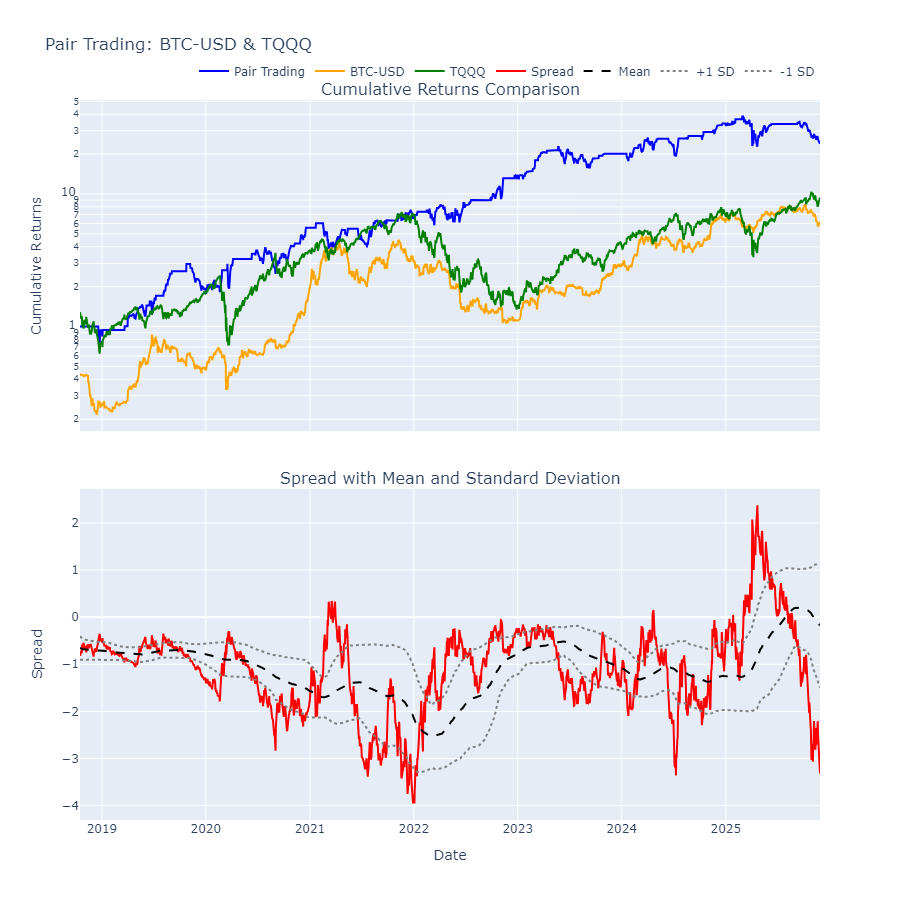
    subplot_titles=('Cumulative Returns Comparison', 'Spread with Mean and Standard Deviation')
)

# 上段: リターン
fig.add_trace(
    go.Scatter(x=cumulative_returns.index, y=cumulative_returns, name='Pair Trading', line=dict(color='blue')),
    row=1, col=1
)
fig.add_trace(
    go.Scatter(x=cum_btc.index, y=cum_btc, name='BTC-USD', line=dict(color='orange')),
    row=1, col=1
)
fig.add_trace(
    go.Scatter(x=cum_tqqq.index, y=cum_tqqq, name='TQQQ', line=dict(color='green')),
    row=1, col=1
)

fig.update_yaxes(type='log', row=1, col=1, title_text='Cumulative Returns')

# 下段: スプレッド
fig.add_trace(
    go.Scatter(x=spread.index, y=spread, name='Spread', line=dict(color='red')),
    row=2, col=1
)
fig.add_trace(
    go.Scatter(x=spread_mean.index, y=spread_mean, name='Mean', line=dict(color='black', dash='dash')),
    row=2, col=1
)
fig.add_trace(
    go.Scatter(x=spread_mean.index, y=spread_mean+spread_std, name='+1 SD', line=dict(color='gray', dash='dot')),
    row=2, col=1
)
fig.add_trace(
    go.Scatter(x=spread_mean.index, y=spread_mean-spread_std, name='-1 SD', line=dict(color='gray', dash='dot')),
    row=2, col=1
)

fig.update_yaxes(title_text='Spread', row=2, col=1)
fig.update_xaxes(title_text='Date', row=2, col=1)

fig.update_layout(
    height=900, width=900,
    showlegend=True,
    legend=dict(orientation="h", yanchor="bottom", y=1.02, xanchor="right", x=1),
    hovermode='x unified',
    title_text="Pair Trading: BTC-USD & TQQQ"
)
fig.show()