Keras学習済みモデルをFine-tuningさせて精度比較

概要

各種Keras学習済みモデルをFruits 360データセットでFine-tuningさせ、クラス分類モデルを構築
モデル精度を比較する

対象モデル

• VGG16
• InceptionV3
• Xception
• MobileNet

Fruits 360
https://www.kaggle.com/moltean/fruits

• KaggleのFruits 360 dataset
• 81クラス、55244枚の画像データセット

実行環境
Google Colaboratory（GPU）

import numpy as np
import pandas as pd
import matplotlib.pyplot as plt
%config InlineBackend.figure_formats = {'png', 'retina'}

import os, cv2, zipfile, io, re, glob
from PIL import Image
from sklearn.model_selection import train_test_split
from keras.applications.vgg16 import VGG16
from keras.applications.inception_v3 import InceptionV3
from keras.applications.inception_resnet_v2 import InceptionResNetV2
from keras.applications.xception import Xception
from keras.models import Model, load_model
from keras.layers.core import Dense
from keras.layers.pooling import GlobalAveragePooling2D
from keras.optimizers import Adam, RMSprop, SGD
from keras.utils.np_utils import to_categorical
from keras.callbacks import ModelCheckpoint, EarlyStopping, TensorBoard, ReduceLROnPlateau
from keras.preprocessing.image import ImageDataGenerator

データ取得

81クラスの内、30クラスの画像を取得。

# ZIP読み込み
z = zipfile.ZipFile('../dataset/fruits-360.zip')

# ラベリングされたディレクトリのみ取得
img_dirs = [ x for x in z.namelist() if re.search("^fruits-360/Training/.*/$", x)]
# 不要な文字列削除
img_dirs = [ x.replace('fruits-360/Training/', '') for x in img_dirs]
img_dirs = [ x.replace('/', '') for x in img_dirs]
img_dirs.sort()

# クラス取得
classes = img_dirs

# クラス数
#num_classes = len(classes)
num_classes = 30

del img_dirs

画像は150にリサイズ後、配列に変換

# 画像サイズ
image_size = 150

# 画像を取得し、配列に変換
def im2array(path):
    X = []
    y = []
    class_num = 0

    for class_name in classes:
        if class_num == num_classes : break
        imgfiles = [ x for x in z.namelist() if re.search("^" + path + class_name + "/.*jpg$", x)]
        for imgfile in imgfiles:
            # ZIPから画像読み込み
            image = Image.open(io.BytesIO(z.read(imgfile)))
            # RGB変換
            image = image.convert('RGB')
            # リサイズ
            image = image.resize((image_size, image_size))
            # 画像から配列に変換
            data = np.asarray(image)
            X.append(data)
            y.append(classes.index(class_name))
        class_num += 1

    X = np.array(X)
    y = np.array(y)
    
    return X, y

trainデータ取得

%%time
X_train, y_train = im2array("fruits-360/Training/")
print(X_train.shape, y_train.shape)

(15094, 150, 150, 3) (15094,)
CPU times: user 14.1 s, sys: 1.56 s, total: 15.7 s
Wall time: 15.9 s

testデータ取得

%%time
X_test, y_test = im2array("fruits-360/Test/")
print(X_test.shape, y_test.shape)

(5060, 150, 150, 3) (5060,)
CPU times: user 8.02 s, sys: 307 ms, total: 8.32 s
Wall time: 8.39 s

del z

# データ型の変換
X_train = X_train.astype('float32')
X_test = X_test.astype('float32')

# 正規化
X_train /= 255
X_test /= 255

# one-hot 変換
y_train = to_categorical(y_train, num_classes = num_classes)
y_test = to_categorical(y_test, num_classes = num_classes)
print(y_train.shape, y_test.shape)

(15094, 30) (5060, 30)

trainデータからvalidデータを分割

X_train, X_valid, y_train, y_valid = train_test_split(
    X_train,
    y_train,
    random_state = 0,
    stratify = y_train,
    test_size = 0.2
)
print(X_train.shape, y_train.shape, X_valid.shape, y_valid.shape) 

(12075, 150, 150, 3) (12075, 30) (3019, 150, 150, 3) (3019, 30)

学習済みモデルの精度比較

Data Augmentation

datagen = ImageDataGenerator(
    featurewise_center = False,
    samplewise_center = False,
    featurewise_std_normalization = False,
    samplewise_std_normalization = False,
    zca_whitening = False,
    rotation_range = 0,
    width_shift_range = 0.1,
    height_shift_range = 0.1,
    horizontal_flip = True,
    vertical_flip = False
)

Callback

# EarlyStopping
early_stopping = EarlyStopping(
    monitor = 'val_loss',
    patience = 10,
    verbose = 1
)

# ModelCheckpoint
weights_dir = './weights/'
if os.path.exists(weights_dir) == False:os.mkdir(weights_dir)
model_checkpoint = ModelCheckpoint(
    weights_dir + "val_loss{val_loss:.3f}.hdf5",
    monitor = 'val_loss',
    verbose = 1,
    save_best_only = True,
    save_weights_only = True,
    period = 3
)

# reduce learning rate
reduce_lr = ReduceLROnPlateau(
    monitor = 'val_loss',
    factor = 0.1,
    patience = 3,
    verbose = 1
)

# log for TensorBoard
logging = TensorBoard(log_dir = "log/")

各種関数定義

# モデル学習
def model_fit():
    hist = model.fit_generator(
        datagen.flow(X_train, y_train, batch_size = 32),
        steps_per_epoch = X_train.shape[0] // 32,
        epochs = 50,
        validation_data = (X_valid, y_valid),
        callbacks = [early_stopping, reduce_lr],
        shuffle = True,
        verbose = 1
    )
    return hist

# モデル保存
model_dir = './model/'
if os.path.exists(model_dir) == False : os.mkdir(model_dir)

def model_save(model_name):
    model.save(model_dir + 'model_' + model_name + '.hdf5')

    # optimizerのない軽量モデルを保存（学習や評価不可だが、予測は可能）
    model.save(model_dir + 'model_' + model_name + '-opt.hdf5', include_optimizer = False)

# 学習曲線をプロット
def learning_plot(title):
    plt.figure(figsize = (18,6))

    # accuracy
    plt.subplot(1, 2, 1)
    plt.plot(hist.history["acc"], label = "acc", marker = "o")
    plt.plot(hist.history["val_acc"], label = "val_acc", marker = "o")
    #plt.yticks(np.arange())
    #plt.xticks(np.arange())
    plt.ylabel("accuracy")
    plt.xlabel("epoch")
    plt.title(title)
    plt.legend(loc = "best")
    plt.grid(color = 'gray', alpha = 0.2)

    # loss
    plt.subplot(1, 2, 2)
    plt.plot(hist.history["loss"], label = "loss", marker = "o")
    plt.plot(hist.history["val_loss"], label = "val_loss", marker = "o")
    #plt.yticks(np.arange())
    #plt.xticks(np.arange())
    plt.ylabel("loss")
    plt.xlabel("epoch")
    plt.title(title)
    plt.legend(loc = "best")
    plt.grid(color = 'gray', alpha = 0.2)

    plt.show()

# モデル評価
def model_evaluate():
    score = model.evaluate(X_test, y_test, verbose = 1)
    print("evaluate loss: {[0]:.4f}".format(score))
    print("evaluate acc: {[1]:.1%}".format(score))

VGG16

base_model = VGG16(
    include_top = False,
    weights = "imagenet",
    input_shape = None
)

# 全結合層の新規構築
x = base_model.output
x = GlobalAveragePooling2D()(x)
x = Dense(1024, activation = 'relu')(x)
predictions = Dense(num_classes, activation = 'softmax')(x)

# ネットワーク定義
model = Model(inputs = base_model.input, outputs = predictions)
print("{}層".format(len(model.layers)))

22層

全22層の内、17層までfreezeさせ、18層以降を学習させる。

# 17層までfreeze
for layer in model.layers[:17]:
    layer.trainable = False
        
# 18層以降、学習させる
for layer in model.layers[17:]:
    layer.trainable = True
    
# layer.trainableの設定後にcompile
model.compile(
    optimizer = Adam(),
    loss = 'categorical_crossentropy',
    metrics = ["accuracy"]
)

%%time
hist = model_fit()

Epoch 1/50
377/377 [==============================] - 98s 260ms/step - loss: 0.4985 - acc: 0.8490 - val_loss: 0.1256 - val_acc: 0.9530
Epoch 2/50
377/377 [==============================] - 96s 255ms/step - loss: 0.0727 - acc: 0.9732 - val_loss: 0.0732 - val_acc: 0.9665
Epoch 3/50
377/377 [==============================] - 96s 255ms/step - loss: 0.0581 - acc: 0.9770 - val_loss: 0.0297 - val_acc: 0.9851

〜省略〜

Epoch 24/50
377/377 [==============================] - 94s 248ms/step - loss: 0.0203 - acc: 0.9871 - val_loss: 0.0218 - val_acc: 0.9834
Epoch 25/50
377/377 [==============================] - 93s 247ms/step - loss: 0.0206 - acc: 0.9854 - val_loss: 0.0218 - val_acc: 0.9834
Epoch 26/50
377/377 [==============================] - 93s 246ms/step - loss: 0.0204 - acc: 0.9864 - val_loss: 0.0218 - val_acc: 0.9834

Epoch 00026: ReduceLROnPlateau reducing learning rate to 1.000000082740371e-08.
Epoch 27/50
377/377 [==============================] - 92s 245ms/step - loss: 0.0203 - acc: 0.9872 - val_loss: 0.0218 - val_acc: 0.9834
Epoch 00027: early stopping
CPU times: user 50min 41s, sys: 4min 41s, total: 55min 22s
Wall time: 42min 35s

learning_plot("VGG16")

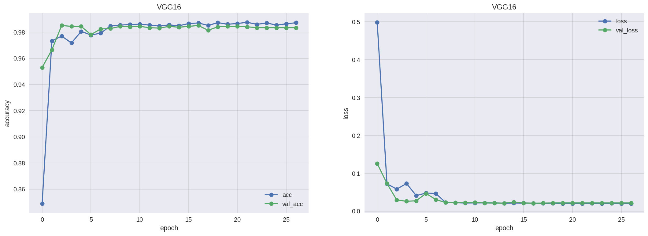
model_evaluate()

5060/5060 [==============================] - 24s 5ms/step
evaluate loss: 0.1116
evaluate acc: 96.1%

model_save("VGG16")

InceptionV3

base_model = InceptionV3(
    include_top = False,
    weights = "imagenet",
    input_shape = None
)

# 全結合層の新規構築
x = base_model.output
x = GlobalAveragePooling2D()(x)
x = Dense(1024, activation = 'relu')(x)
predictions = Dense(num_classes, activation = 'softmax')(x)

# ネットワーク定義
model = Model(inputs = base_model.input, outputs = predictions)
print("{}層".format(len(model.layers)))

314層

全314層の内、249層までfreezeさせ、250層以降を学習させる。

# 249層までfreeze
for layer in model.layers[:249]:
    layer.trainable = False
    
    # Batch Normalization の freeze解除
    if layer.name.startswith('batch_normalization'):
        layer.trainable = True

#250層以降、学習させる
for layer in model.layers[249:]:
    layer.trainable = True
    
# layer.trainableの設定後にcompile
model.compile(
    optimizer = Adam(),
    loss = 'categorical_crossentropy',
    metrics = ["accuracy"]
)

%%time
hist=model_fit()

Epoch 1/50
377/377 [==============================] - 148s 394ms/step - loss: 0.3223 - acc: 0.9127 - val_loss: 0.0609 - val_acc: 0.9748
Epoch 2/50
377/377 [==============================] - 129s 343ms/step - loss: 0.0962 - acc: 0.9684 - val_loss: 0.0469 - val_acc: 0.9781
Epoch 3/50
377/377 [==============================] - 129s 343ms/step - loss: 0.0676 - acc: 0.9756 - val_loss: 0.0365 - val_acc: 0.9821

〜省略〜

Epoch 19/50
377/377 [==============================] - 129s 341ms/step - loss: 0.0225 - acc: 0.9859 - val_loss: 0.0210 - val_acc: 0.9844
Epoch 20/50
377/377 [==============================] - 128s 340ms/step - loss: 0.0235 - acc: 0.9857 - val_loss: 0.0210 - val_acc: 0.9844
Epoch 21/50
377/377 [==============================] - 129s 342ms/step - loss: 0.0210 - acc: 0.9865 - val_loss: 0.0210 - val_acc: 0.9848

Epoch 00021: ReduceLROnPlateau reducing learning rate to 1.000000082740371e-08.
Epoch 00021: early stopping
CPU times: user 1h 8min 40s, sys: 9min 16s, total: 1h 17min 56s
Wall time: 45min 28s

learning_plot("InceptionV3")

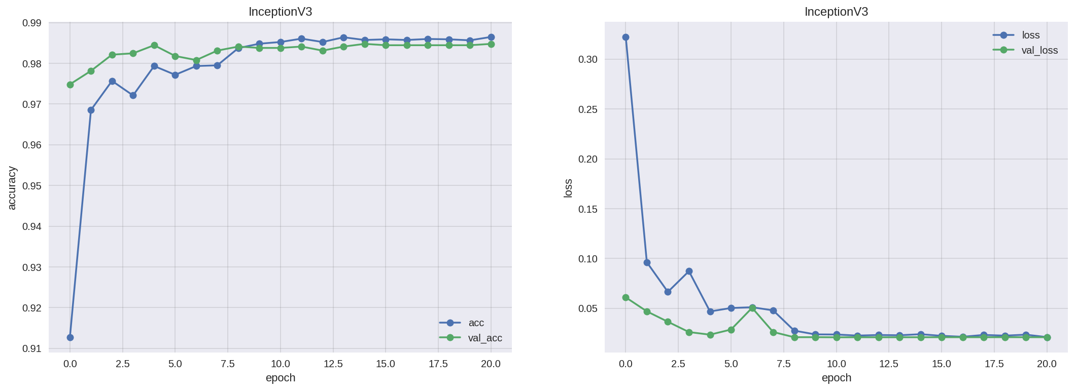
model_evaluate()

5060/5060 [==============================] - 15s 3ms/step
evaluate loss: 0.2082
evaluate acc: 96.5%

model_save("InceptionV3")

VGG16に比べ、accuracyは良くなったが、代わりにlossが増え、必ずしも精度が高いとは言い切れない。

Xception

base_model = Xception(
    include_top = False,
    weights = "imagenet",
    input_shape = None
)

# 全結合層の新規構築
x = base_model.output
x = GlobalAveragePooling2D()(x)
x = Dense(1024, activation = 'relu')(x)
predictions = Dense(num_classes, activation = 'softmax')(x)

# ネットワーク定義
model = Model(inputs = base_model.input, outputs = predictions)
print("{}層".format(len(model.layers)))

135層

全135層の内、108層までfreezeさせ、109層以降を学習させる。

#108層までfreeze
for layer in model.layers[:108]:
    layer.trainable = False
    
    # Batch Normalization の freeze解除
    if layer.name.startswith('batch_normalization'):
        layer.trainable = True
    if layer.name.endswith('bn'):
        layer.trainable = True
        
#109層以降、学習させる
for layer in model.layers[108:]:
    layer.trainable = True
    
# layer.trainableの設定後にcompile
model.compile(
    optimizer = Adam(),
    loss = 'categorical_crossentropy',
    metrics = ["accuracy"]
)

%%time
hist = model_fit()

Epoch 1/50
377/377 [==============================] - 172s 455ms/step - loss: 0.2736 - acc: 0.9318 - val_loss: 0.0859 - val_acc: 0.9669
Epoch 2/50
377/377 [==============================] - 162s 429ms/step - loss: 0.1284 - acc: 0.9626 - val_loss: 0.0389 - val_acc: 0.9824
Epoch 3/50
377/377 [==============================] - 161s 426ms/step - loss: 0.0882 - acc: 0.9724 - val_loss: 0.0275 - val_acc: 0.9824

〜省略〜

Epoch 16/50
377/377 [==============================] - 161s 427ms/step - loss: 0.0220 - acc: 0.9862 - val_loss: 0.0232 - val_acc: 0.9838
Epoch 17/50
377/377 [==============================] - 161s 427ms/step - loss: 0.0219 - acc: 0.9864 - val_loss: 0.0229 - val_acc: 0.9841
Epoch 18/50
377/377 [==============================] - 161s 427ms/step - loss: 0.0228 - acc: 0.9859 - val_loss: 0.0226 - val_acc: 0.9844

Epoch 00018: ReduceLROnPlateau reducing learning rate to 1.0000000656873453e-06.
Epoch 19/50
377/377 [==============================] - 161s 427ms/step - loss: 0.0229 - acc: 0.9865 - val_loss: 0.0226 - val_acc: 0.9844
Epoch 00019: early stopping
CPU times: user 1h 41s, sys: 12min 51s, total: 1h 13min 33s
Wall time: 51min 20s

learning_plot("Xception")

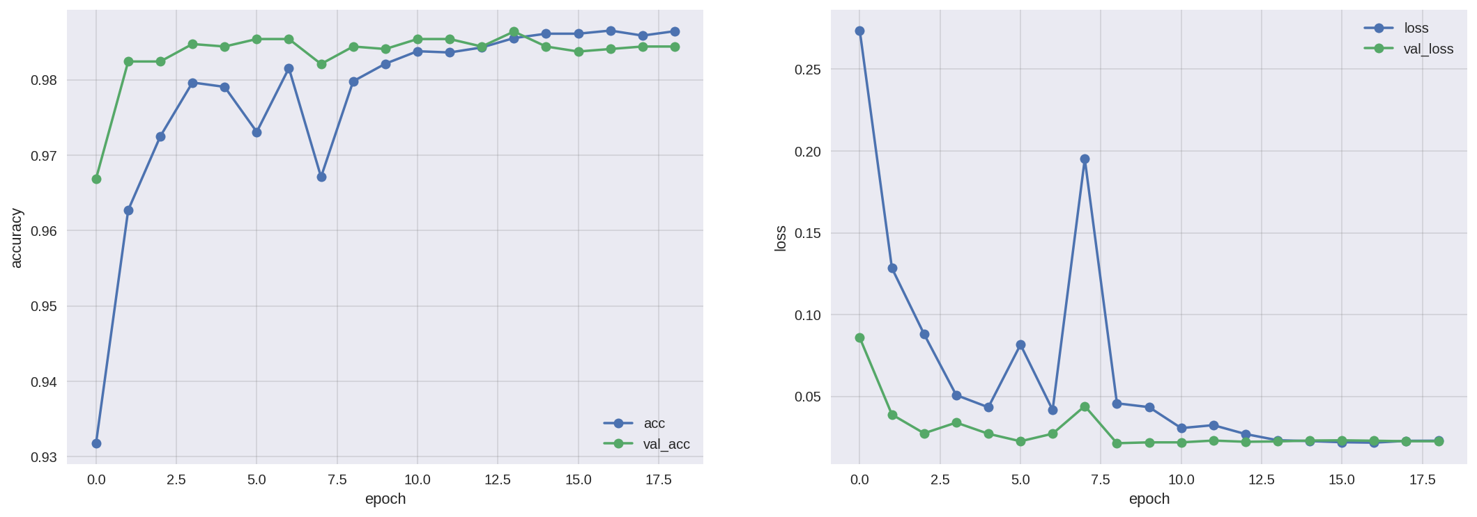
model_evaluate()

5060/5060 [==============================] - 25s 5ms/step
evaluate loss: 0.0977
evaluate acc: 97.7%

model_save("Xception")

VGG16やInceptionV3に比べ、accuracy、lossともに精度が高い。

MobileNet

base_model = MobileNet(
    include_top = False,
    weights = "imagenet",
    input_shape = None
)

# 全結合層の新規構築
x = base_model.output
x = GlobalAveragePooling2D()(x)
x = Dense(1024, activation = 'relu')(x)
predictions = Dense(num_classes, activation = 'softmax')(x)

# ネットワーク定義
model = Model(inputs = base_model.input, outputs = predictions)
print("{}層".format(len(model.layers)))

90層

全90層の内、72層までfreezeさせ、73層以降を学習させる。

# 72層までfreeze
for layer in model.layers[:72]:
    layer.trainable = False
    
    # Batch Normalization の freeze解除
    if "bn" in layer.name:
        layer.trainable = True

#73層以降、学習させる
for layer in model.layers[72:]:
    layer.trainable = True
    
# layer.trainableの設定後にcompile
model.compile(
    optimizer = Adam(),
    loss = 'categorical_crossentropy',
    metrics = ["accuracy"]
)

%%time
hist = model_fit()

Epoch 1/50
377/377 [==============================] - 92s 244ms/step - loss: 0.0857 - acc: 0.9759 - val_loss: 0.2791 - val_acc: 0.9543
Epoch 2/50
377/377 [==============================] - 79s 210ms/step - loss: 0.0938 - acc: 0.9746 - val_loss: 0.5770 - val_acc: 0.9232
Epoch 3/50
377/377 [==============================] - 80s 212ms/step - loss: 0.0881 - acc: 0.9758 - val_loss: 0.1943 - val_acc: 0.9629

〜省略〜

Epoch 19/50
377/377 [==============================] - 82s 217ms/step - loss: 0.0209 - acc: 0.9859 - val_loss: 0.0212 - val_acc: 0.9854
Epoch 20/50
377/377 [==============================] - 81s 216ms/step - loss: 0.0204 - acc: 0.9867 - val_loss: 0.0212 - val_acc: 0.9858
Epoch 21/50
377/377 [==============================] - 81s 216ms/step - loss: 0.0197 - acc: 0.9867 - val_loss: 0.0212 - val_acc: 0.9854

Epoch 00021: ReduceLROnPlateau reducing learning rate to 1.0000001111620805e-07.
Epoch 22/50
377/377 [==============================] - 82s 216ms/step - loss: 0.0216 - acc: 0.9869 - val_loss: 0.0212 - val_acc: 0.9858
Epoch 00022: early stopping
CPU times: user 42min 23s, sys: 3min 30s, total: 45min 53s
Wall time: 29min 59s

learning_plot("MobileNet")

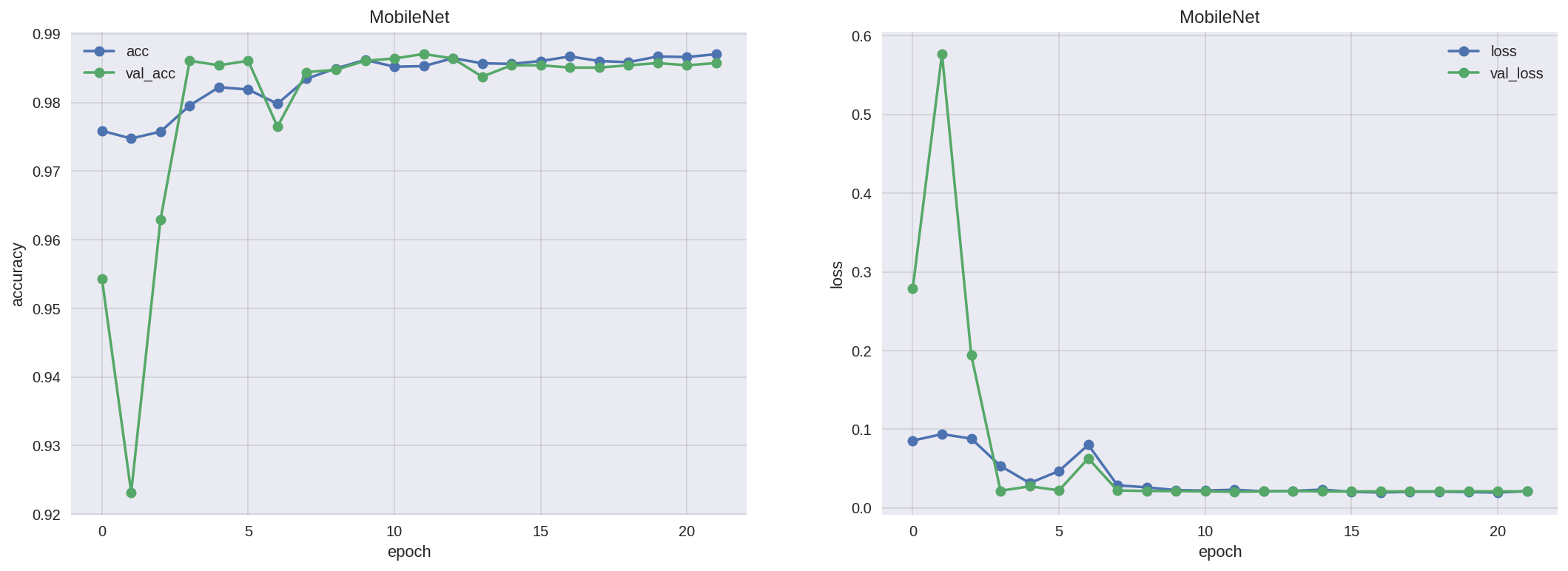
model_evaluate()

5060/5060 [==============================] - 7s 1ms/step
evaluate loss: 0.1705
evaluate acc: 97.6%

model_save("MobileNet")

エポックごとの学習速度が、最も早い。
データセットに依るのだろうが、accuracyがVGG16やInceptionV3よりも高く、Xceptionに近い値を計測したことが驚きである。

モデルの精度比較

accuracy
Xception ≒ MobileNet > Inception > VGG16
loss
Xception < VGG16 < MobileNet < Inception
各エポックごとの学習速度
MobileNet > VGG16 > Inception > Xception

今後はAWSを使って、InceptionResNetV2モデルを検証してみたい。

モデル予測

最後に最も精度が高かったXceptionモデルで、testデータを予測。

モデル読み込み

model = load_model(model_dir + 'model_Xception-opt.hdf5', compile = False)

# 相互のインデックスを対応させながらシャッフル
def shuffle_samples(X, y):
    zipped = list(zip(X, y))
    np.random.shuffle(zipped)
    X_result, y_result = zip(*zipped)
    return np.asarray(X_result), np.asarray(y_result)
X_test, y_test = shuffle_samples(X_test, y_test)

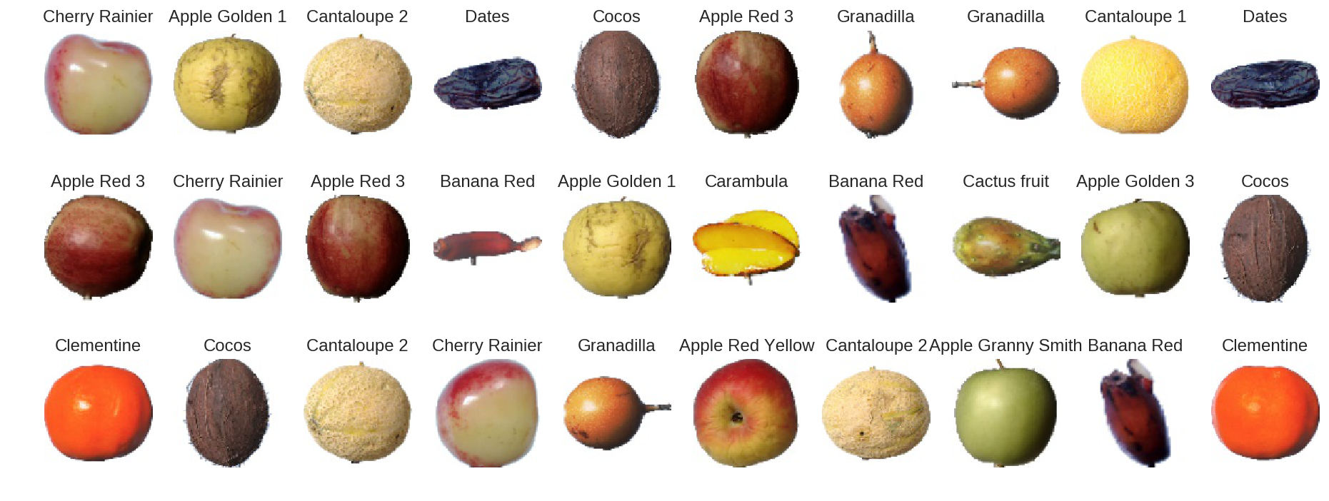
testデータ30件の画像と正解ラベルを出力

# testデータ30件の正解ラベル
true_classes = np.argmax(y_test[0:30], axis = 1)

# testデータ30件の画像と正解ラベルを出力
plt.figure(figsize = (16, 6))
for i in range(30):
    plt.subplot(3, 10, i + 1)
    plt.axis("off")
    plt.title(classes[true_classes[i]])
    plt.imshow(X_test[i])
plt.show()

testデータ30件の画像と予測ラベル・予測確率を出力

# testデータ30件の予測ラベル
pred_classes = np.argmax(model.predict(X_test[0:30]), axis = 1)

# testデータ30件の予測確率
pred_probs = np.max(model.predict(X_test[0:30]), axis = 1)
pred_probs = ['{:.4f}'.format(i) for i in pred_probs]

# testデータ30件の画像と予測ラベル・予測確率を出力
plt.figure(figsize = (16, 6))
for i in range(30):
    plt.subplot(3, 10, i + 1)
    plt.axis("off")
    if pred_classes[i] == true_classes[i]:
        plt.title(classes[pred_classes[i]] + '\n' + pred_probs[i])
    else:
        plt.title(classes[pred_classes[i]] + '\n' + pred_probs[i], color = "red")
    plt.imshow(X_test[i])
plt.show()

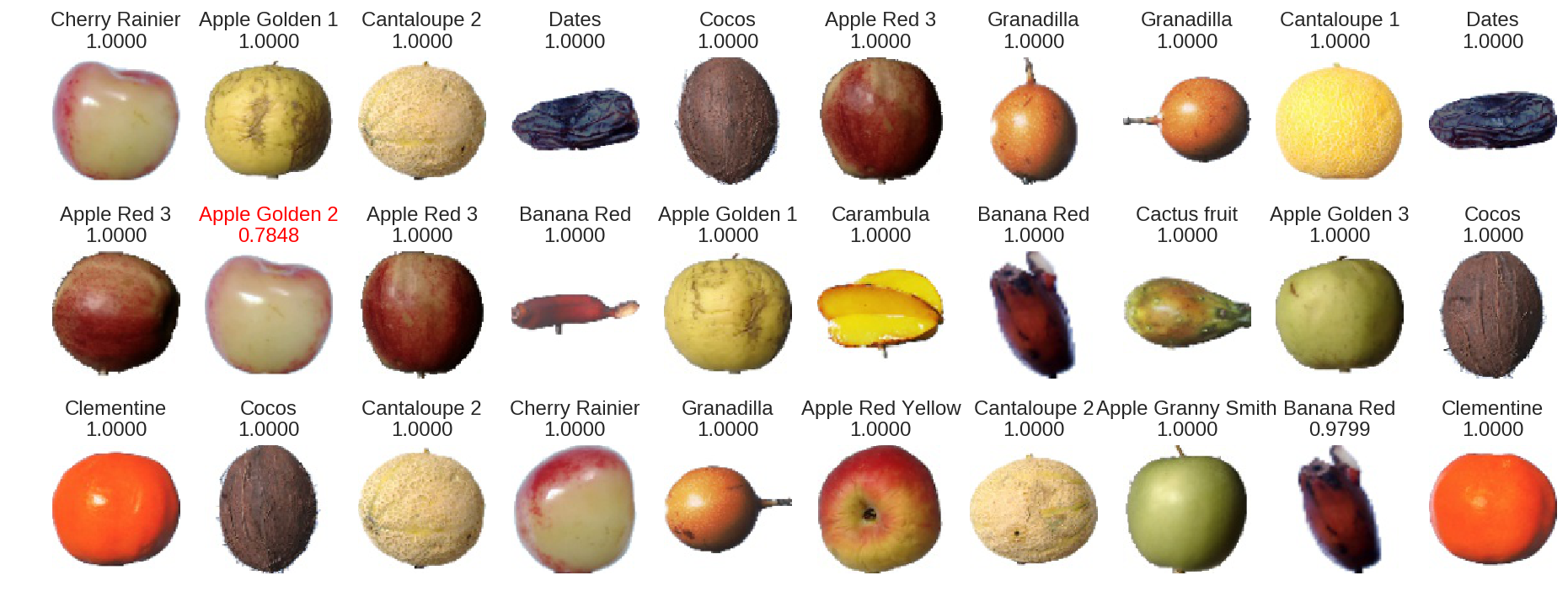
高い確率でクラス分類できているかなと。