Language: 日本語 · English

A Metrology Museum on Paper — The Instrument Wing (sensors and instruments reproduced from physics)

One wing of A Metrology Museum on Paper — the entrance, where the other wings, the glossary and the thesis live.

32 exhibits hang in this wing. The numbers are accession numbers: they do not change when an exhibit moves or when an article is split.

The "Ops used" line under each exhibit links to that op's note (type contract, pitfalls, figures, a runnable Studio program): Operator catalogue / Op notes index.

The Instrument Wing — From Raw Output to Instrument-Specific Failure

It is easy to borrow an instrument's name and produce a convenient image. The 32 exhibits in this room instead build raw output from photons, electrons, interference, heat diffusion, scanning and ray tracing, then carry that output through to the quantity normally reported.

The same range fails differently in iToF and dToF through multipath and pile-up; the same particles read at different diameters in SEM and TEM. More TDI stages reveal dark defects while accumulating each synchronisation error across all stages. A model that omits the instrument physics cannot reproduce where the instrument breaks.

Every exhibit is gated by a closed form, public measurement or independent implementation. The aim is not to claim a complete substitute for hardware. It is to state which physics is present and which is still absent, then find when the reported measurement stops being trustworthy before touching the instrument.

No.2026.010 —— Where CT Reconstruction Starts to Break as Projections Are Removed

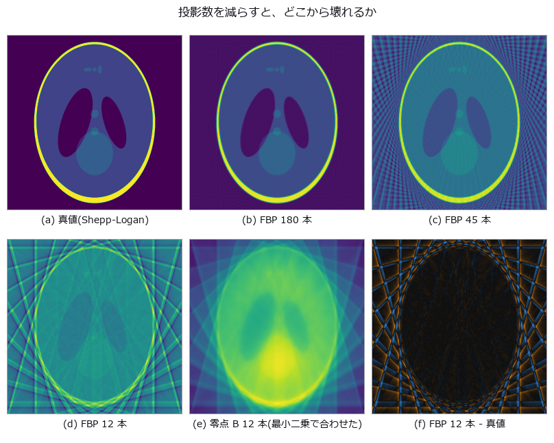
↑ Where CT Reconstruction Starts to Break as Projections Are Removed ―― Shepp-Logan re-imaged with 180 down to 12 projections, FBP placed beside two nulls: a blank image and unfiltered back-projection. With 12 projections FBP (RMSE 0.2576) is worse than the blank image (0.2420). A check that never looks at the reconstruction — the row sums of the sinogram — caught a -3.34 % mass loss that RMSE could not see; fixing the ramp filter's DC bin brought it to -0.0099 %.

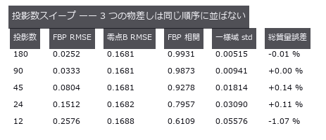
↑ The measurement ―― RMSE で見ると 12 本は空白画像 0.2420 より悪い。相関とストリークは別のことを言う。 (figure labels are in Japanese; the numbers are the same)

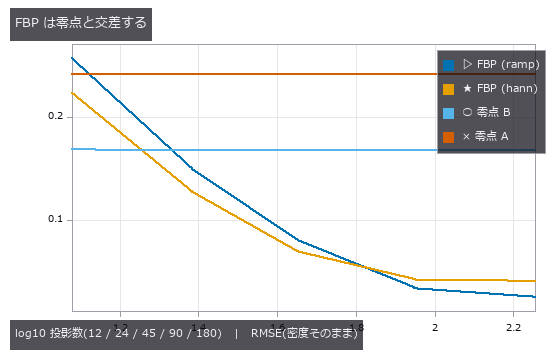
↑ 零点 A = 空白画像、零点 B = 無フィルタ逆投影(どちらも水平・ほぼ水平)。

py -3.11 examples/poc_ct_fidelity.py

Source: examples/poc_ct_fidelity.py

This run produced 3 figures in total - see them all

Ops used (notes): backproject_sinogram · ellipse_phantom · ellipse_sinogram · filtered_backprojection · projection_angles · radon_transform · rmse · ssim · stat_correlation

No.2026.016 —— Ranging by Counting Photons — How Many for How Many Millimetres?

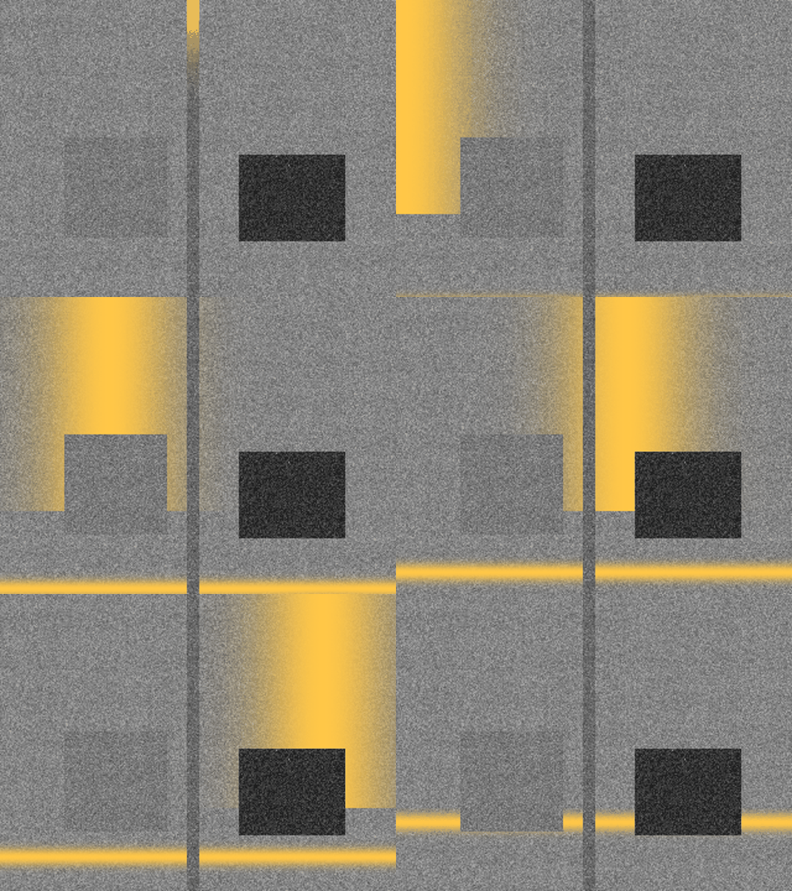
↑ Ranging by Counting Photons — How Many for How Many Millimetres? ―― The lead figure is a 48-frame, 576 x 432 light-front video. An amber light band from a display window widened to 7 % of the depth span crosses from near to far over a grey return-amplitude image stretched from the 1st to 99.5th percentiles with gamma 0.7. A second figure labels an 8x flying-pixel crop, corner bowing and dark-object noise.

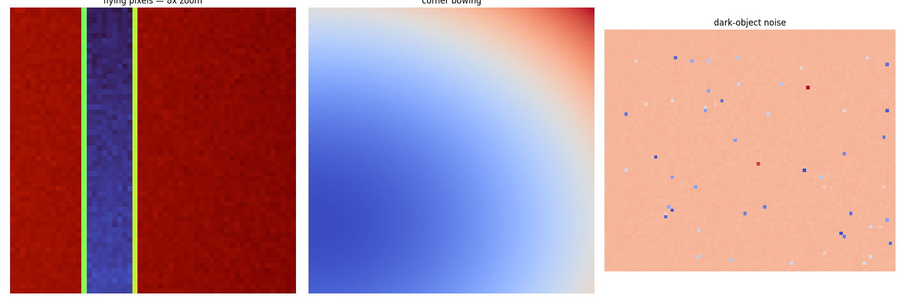
↑ The measurement ―― Flying pixels (8x crop), systematic corner bowing and dark-object range noise shown at a readable scale.

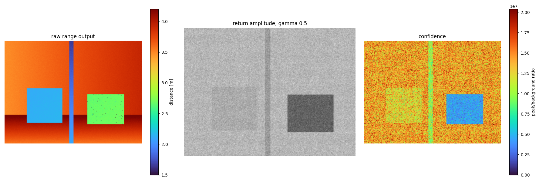
↑ 距離出力｜反射振幅（γ=0.5）｜ピーク/背景比。

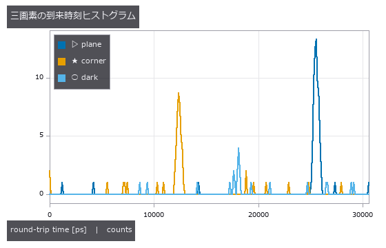
↑ 平面、角、暗い物体。

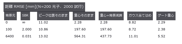
↑ 背景が無ければ素の重心で足りる。

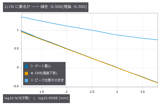
↑ ゲート重心は CRB に寄り添って落ちる。

py -3.11 examples/poc_dtof_ranging.py

Source: examples/poc_dtof_ranging.py

This run produced 8 figures in total - see them all

Ops used (notes): dtof_cube_depth · dtof_cube_simulate · dtof_depth · gaussian · median · spad_deadtime_apply · tcspc_background_subtract · tcspc_coates_correct · tcspc_simulate

No.2026.022 —— How Accurately a White-Light Interferometer Measures a Nanometre Step

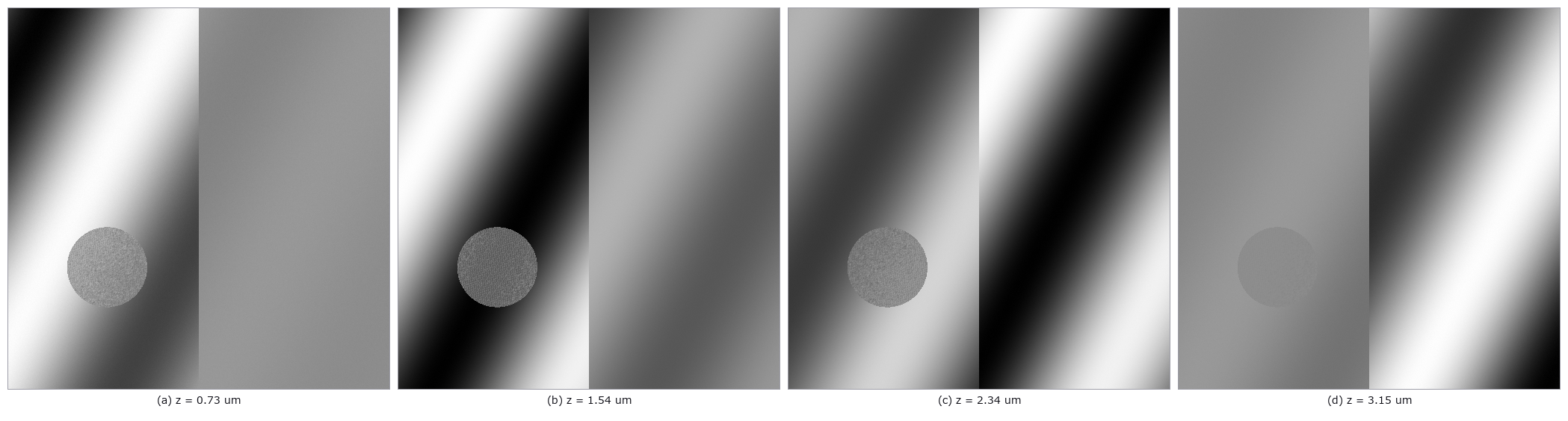
↑ How Accurately a White-Light Interferometer Measures a Nanometre Step ―― A synthesised coherence-scanning stack with steps of 50 to 500 nm measured back. At 1 % noise the bias stays within 2.4 nm and the standard deviation within 14.1 nm, almost independent of step height. The null (envelope's maximum sample) errs by exactly half the scan step, and at 0.14 µm, just inside the Nyquist ceiling of 0.15 µm, the noise-free error is already +14.1 nm.

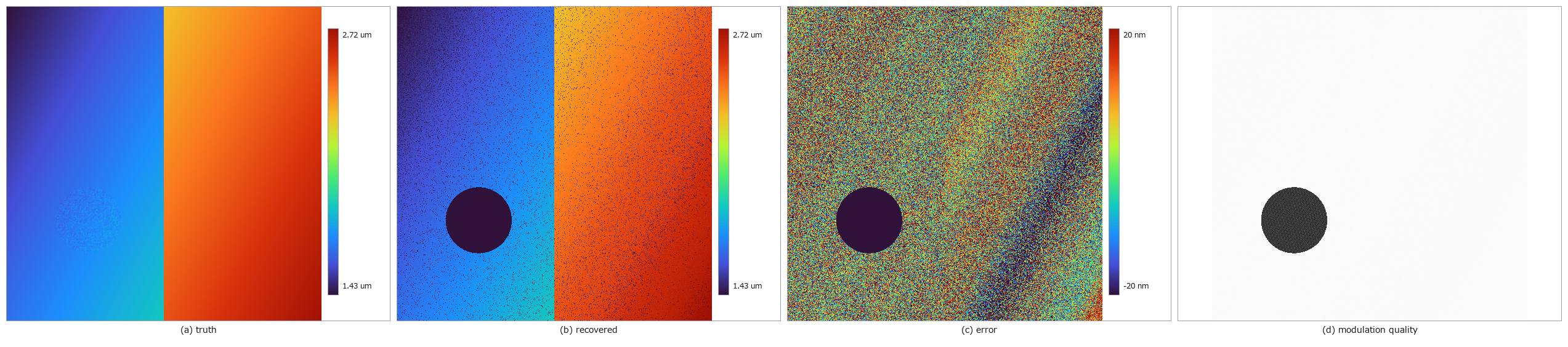
↑ The measurement ―― Truth, recovered height, error and low-modulation dropout map; pseudo-colour bars carry units. (figure labels are in Japanese; the numbers are the same)

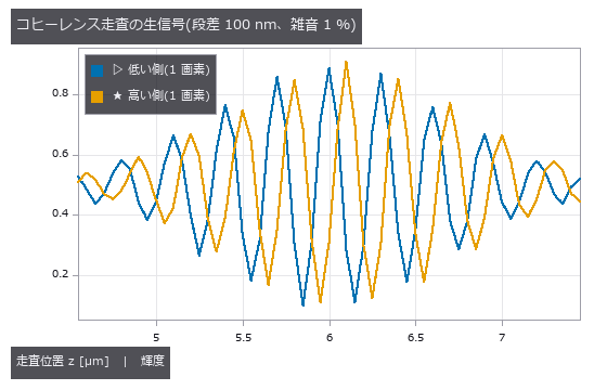
↑ 包絡線の中心が段差ぶんずれる。

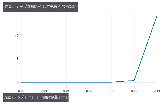
↑ 0.02〜0.12 µm は 0.05 nm 以内で平ら。

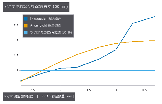
↑ centroid は散らばりが gaussian の 1/3〜1/5 なのに総合誤差では上に来る。

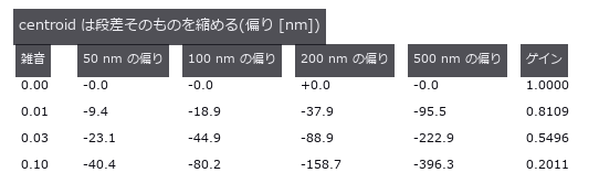
↑ 4 種の段差でゲインが揃う = オフセットではなく倍率の誤差。

↑ The animation ―― 48 raw uint8 coherence-scan frames; the localized envelope sweeps over the tilted step.

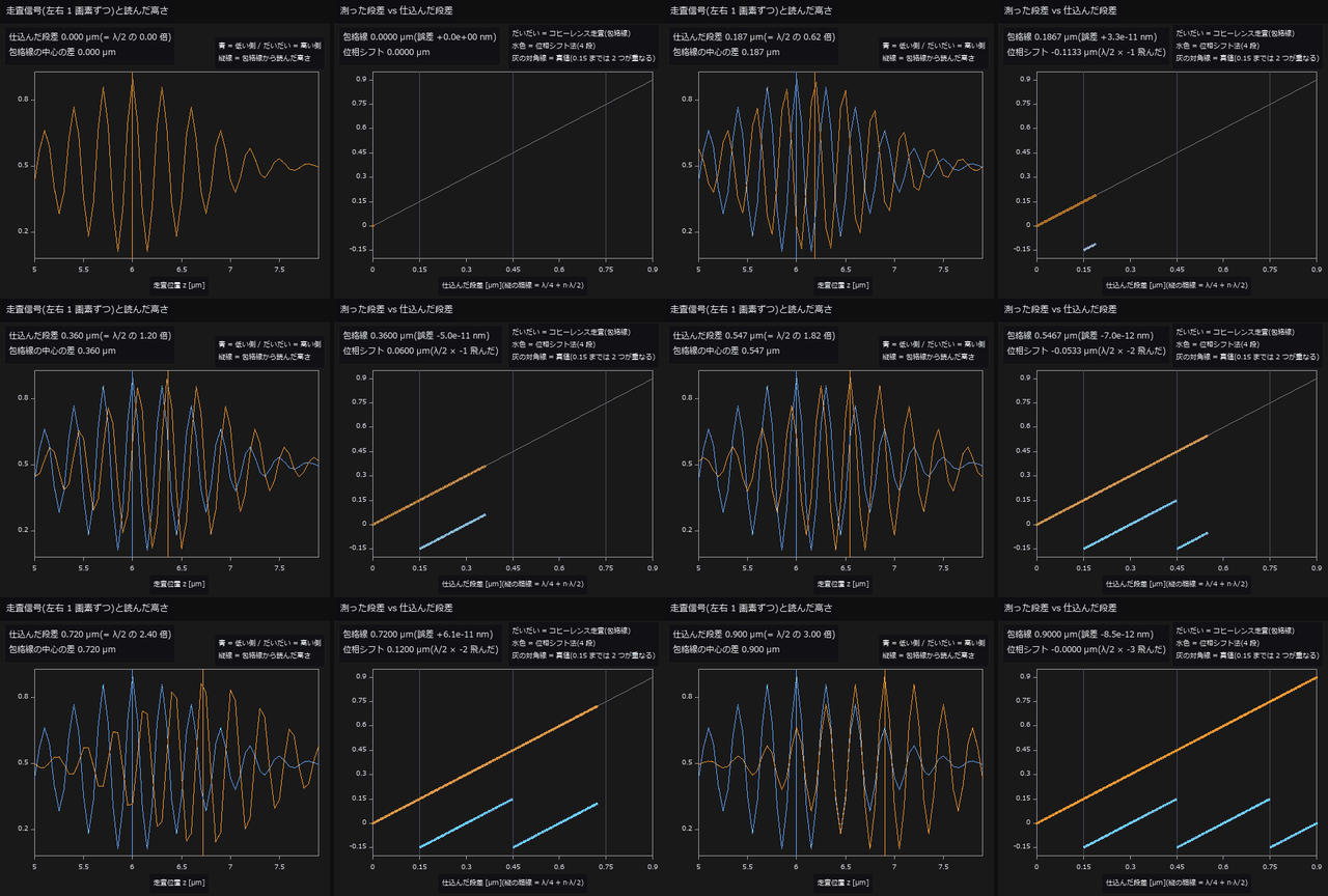
↑ The animation ―― 動画(148 コマ): 仕込む段差を 0 → 0.90 µm へ連続に増やし、同じ表面を 2 つの方法で測る(雑音なし)。左は低い側・高い側 1 画素ずつのコヒーレンス走査の信号で、縦線は csi_height_map(gaussian)が包絡線から読んだ高さ。右は測った段差 vs 仕込んだ段差。包絡線(だいだい)は全域で対角線に乗り、誤差は最大 8.5e-11 nm —— 包絡線には周期が無いので巻き戻らない。位相シフト法(水色、4 段)は段差 0.153 µm(λ/4 = 0.150 µm の直後)で初めて λ/2 ぶん飛び、以後 λ/2 ごとに鋸の歯になる。

py -3.11 examples/poc_interferometry_step.py

Source: examples/poc_interferometry_step.py

This run produced 8 figures in total - see them all

Ops used (notes): axes_frame · axes_transform · color_bar · csi_contrast_map · csi_design · csi_height_map · csi_stack_simulate · decode_fringe · gaussian · plot_series · synthesize_fringes · text_box · ticks

No.2026.023 —— Depth From a Light Field — A Light Field of Known Depth, Confronted With Its Nulls

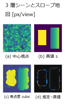
↑ Depth From a Light Field — A Light Field of Known Depth, Confronted With Its Nulls ―― A 9×9 light field rendered by analytic inverse mapping, with focus-measure, EPI-slope and two-view block matching scored against the true slope map. The winner beats the constant null by 22x, but beats two-view matching — which uses only 2 of the 81 views — by just 1.6x, and only with cubic interpolation. The default linear interpolation snaps to integer slopes, reading a true 1.30 as 1.4750 (11.9 % in depth).

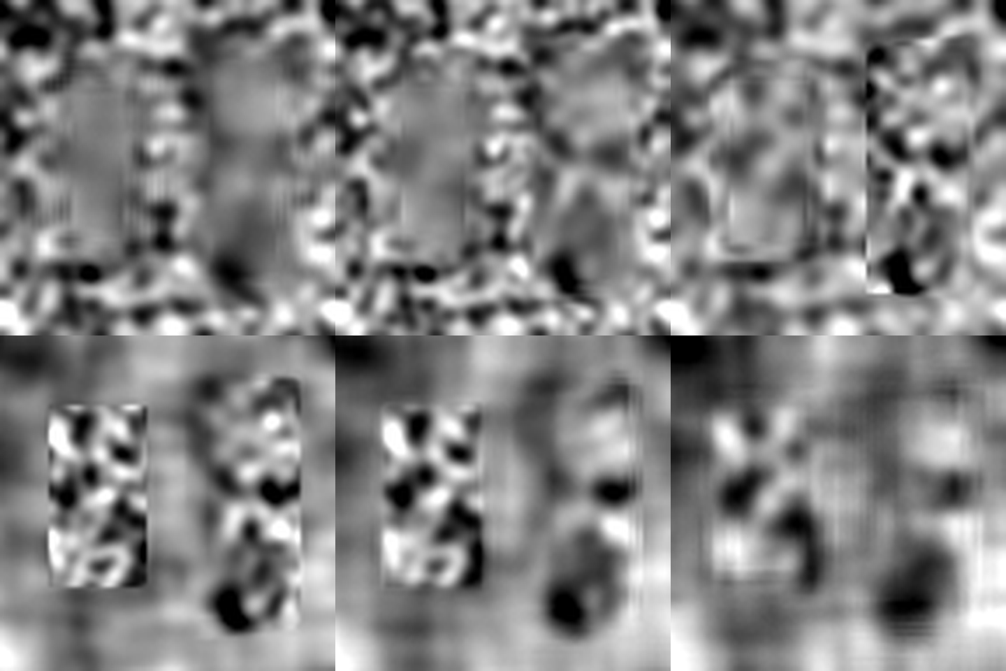
↑ The measurement ―― 9 by 9 sub-aperture views; disparity is in pixels per adjacent view. (figure labels are in Japanese; the numbers are the same)

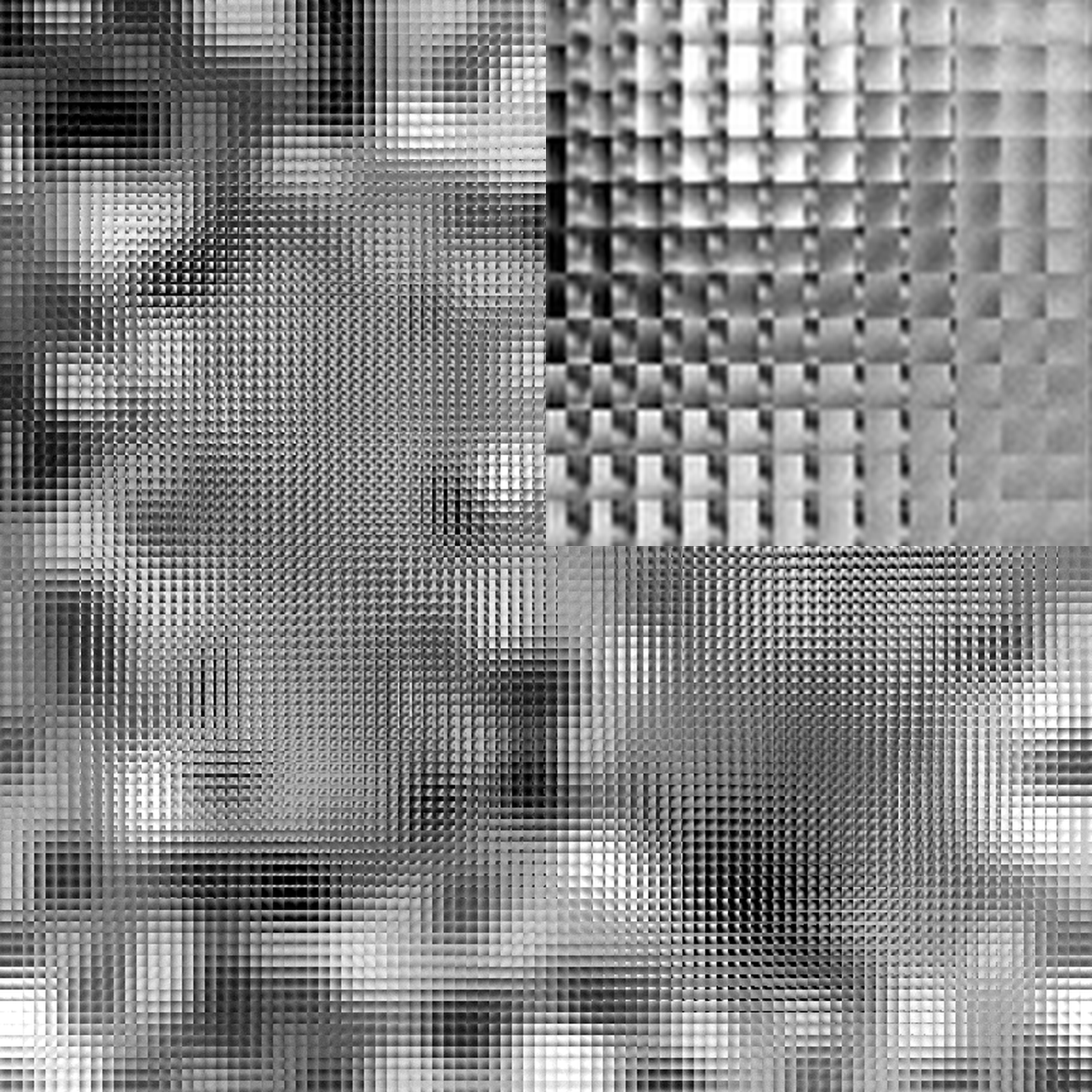
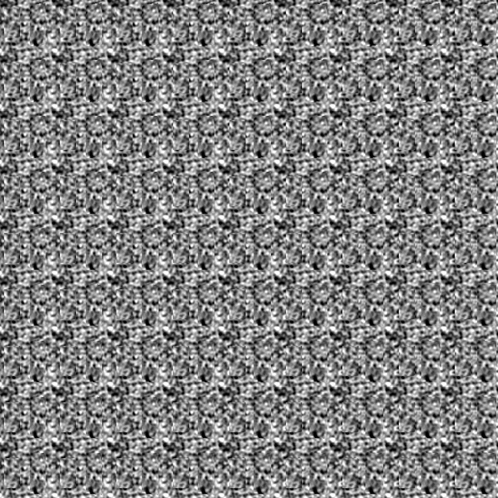
↑ Raw micro-image array with an 8-times-area centre inset; display resize uses Lanczos filtering.

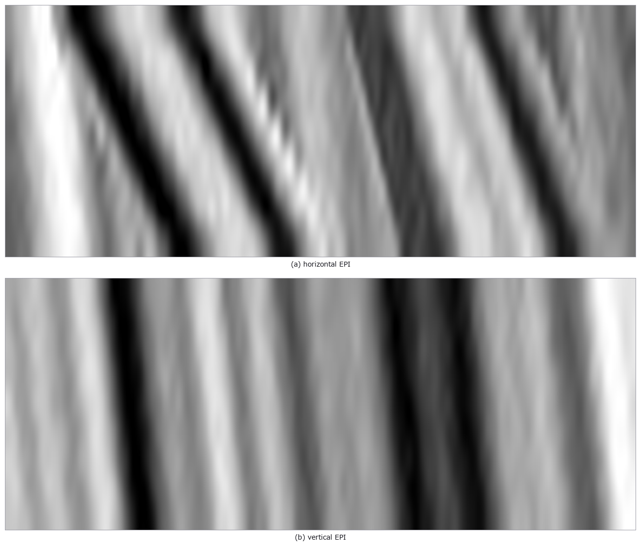
↑ Slanted EPI lines encode disparity in px/view; benchmark format is 9 by 9 views.

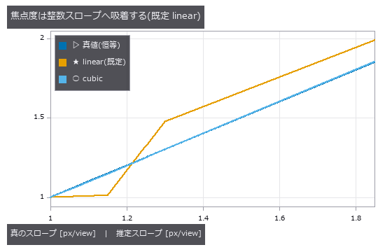
↑ linear は 1.08/1.15 を 1.0 へ、1.85 を 2.0 側へ引く。

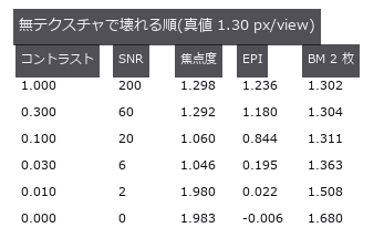
↑ EPI は SNR 20 で既に -35 %。

↑ The animation ―― Twenty-four uint8 refocus frames, 0 to 3 px/view.

py -3.11 examples/poc_lightfield_depth.py

Source: examples/poc_lightfield_depth.py

This run produced 12 figures in total - see them all

Ops used (notes): color_bar · lf_depth_from_focus · lf_disparity_to_depth · lf_epi · lf_epi_slope · lf_refocus · lf_to_mla

No.2026.033 —— Stripping Specular Reflection With Polarisation — Truth From the Fresnel Equations

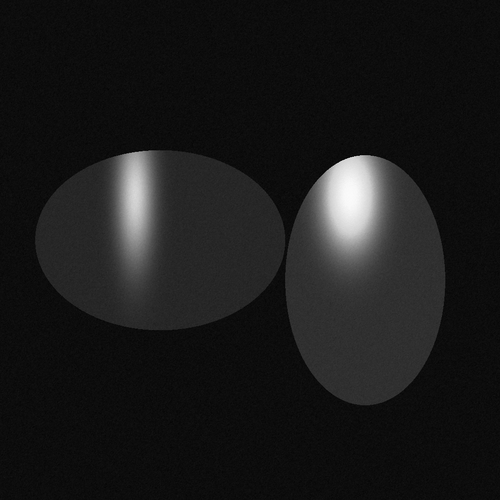
↑ Stripping Specular Reflection With Polarisation — Truth From the Fresnel Equations ―― Diffuse and specular components synthesised as s/p terms with the degree of polarisation from the Fresnel equations, and the separation scored against them. At 20 degrees of incidence the polarisation method wins by only 1.2x. The diffuse error matches the closed form R_p·E exactly and vanishes at the Brewster angle of 56.31 degrees — the diffuse term of polarization_separate is systematically high by that amount.

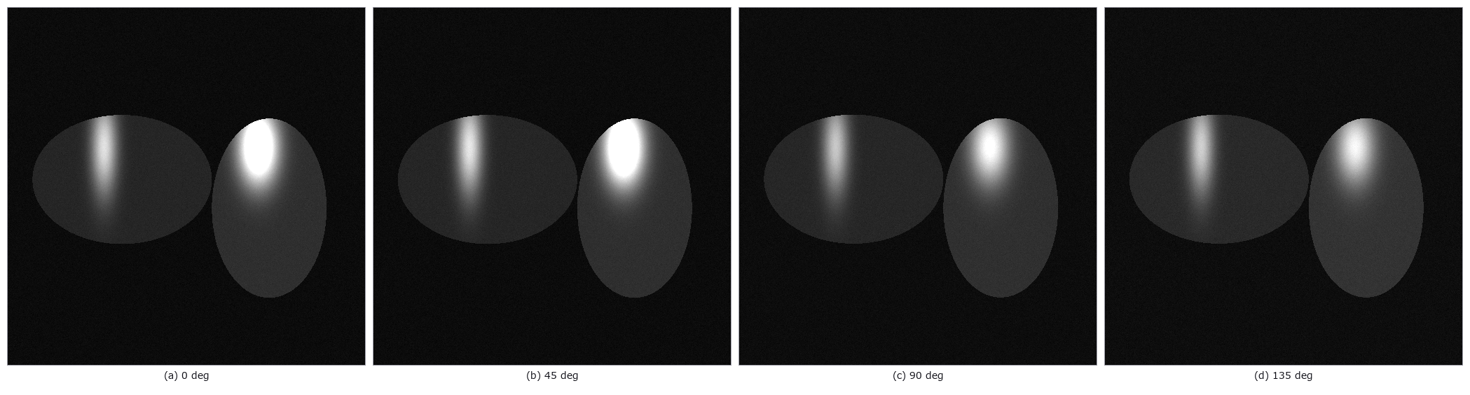
↑ The measurement ―― Half-resolution analyzer samples separated from the mosaic (one quarter of the pixels each). (figure labels are in Japanese; the numbers are the same)

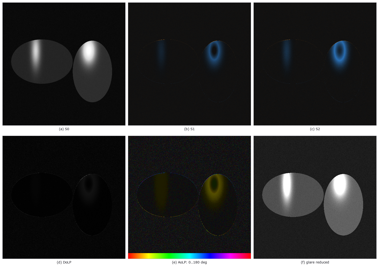
↑ Stokes fields, polarization degree, hue-wheel angle and the minimum-polarized component.

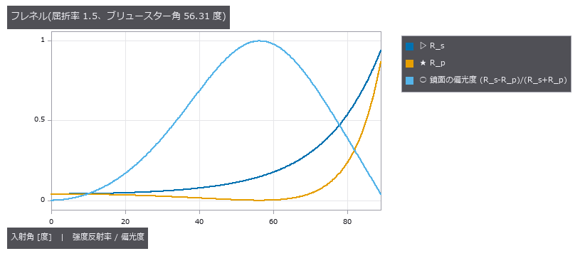
↑ R_p がブリュースター角で 0 を横切る。

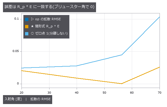
↑ 実測と閉形式が重なる。

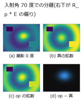
↑ 残差はローブと同じ形。

py -3.11 examples/poc_polarization_specular.py

Source: examples/poc_polarization_specular.py

This run produced 7 figures in total - see them all

Ops used (notes): fresnel_reflectance · polarization_dolp_map · polarization_render · polarization_separate · polarization_stokes · rmse

No.2026.078 —— Drone Thermography of a PV Plant — You Think You Are Measuring Temperature Difference, but You Are Measuring Wind and Viewing Angle

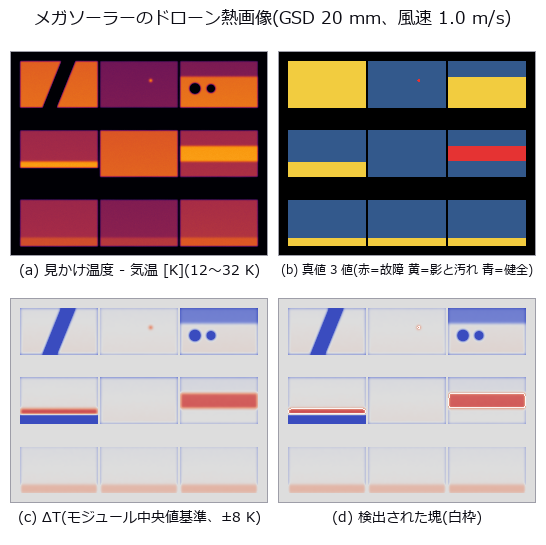
↑ Drone Thermography of a PV Plant — You Think You Are Measuring Temperature Difference, but You Are Measuring Wind and Viewing Angle ―― A megawatt PV array synthesised from a closed-form steady-state heat balance, seeded with known electrical faults (an in-cell hotspot, a bypassed string) and with real-but-not-electrical temperature differences (shading, soiling). A hotspot dissipating 320 W/m² is 11.20 K before dilution yet reaches the camera as 4.23 K — and the dilution comes not from the lateral conduction we expected (x0.960) but from the camera (x0.511). A control scene containing no electrical fault at all still raises 6 blobs when the whole-image mean is the reference (1 healthy, 5 non-fault). The cliff is set by the minimum-area gate rather than the threshold: the hotspot disappears at 1.0 m/s of wind, matching the area-based prediction of 1.1 m/s while the peak-based prediction of 3.0 m/s is wrong. Row-to-row shading warms the sunlit cells of the same string by +4.68 K, only 0.87 K away from the genuine string fault at +5.55 K.

↑ The measurement ―― 「偽」= 故障でも影でも汚れでもない場所に出た塊。しきい値 3.0 K、風速 1.0 m/s。 (figure labels are in Japanese; the numbers are the same)

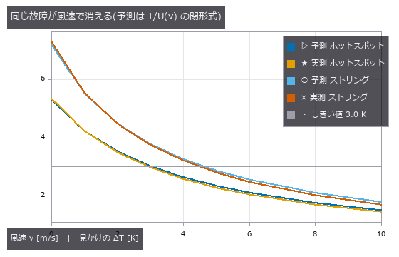
↑ U(v) = 1.75·(5.7 + 3.8v + h_rad)。

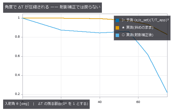
↑ ε(θ) は Fresnel(等価屈折率 1.8)。

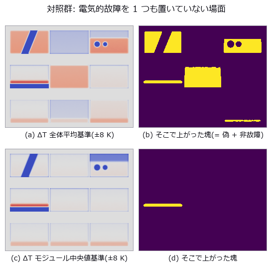
↑ 上段の塊はすべて偽か非故障の温度差。

↑ Module-level correction preserves the detection chapters and their thresholds.

py -3.11 examples/poc_pv_thermal_survey.py

Source: examples/poc_pv_thermal_survey.py

This run produced 10 figures in total - see them all

Ops used (notes): beer_lambert_transmittance · blob_features · blob_label · blob_select · color_bar · fresnel_dielectric · gauss_filter · median · overlay_mask · surface_form_remove · volume_downsample · warp_by_plane · zoom_image_factor

No.2026.113 —— A Thermal Image Is Not a Temperature Image — Emissivity, Reflection, and an Uncertainty That Does Not Add

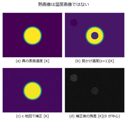
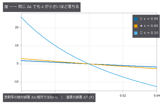
↑ A Thermal Image Is Not a Temperature Image — Emissivity, Reflection, and an Uncertainty That Does Not Add ―― Take a thermal camera's digital numbers all the way back to temperature, with the truth planted: L = tau [ eps L_bb(T_obj) + (1-eps) L_bb(T_refl) ] + (1-tau) L_bb(T_atm). The floor is measured first — 1.75e-06 K round trip, 6.28e-03 K with quantisation, 2.71e-02 K with NETD — and re-measured off the calibration knots, because at exactly 350.0 K the error came out identically zero and calling that a floor would be a lie. The closed form was printed before measuring, and it was wrong: the naive Planck exponent n = c2/(lambda T) misses the numerical derivative by up to 16.6 %, and the culprit is not the choice of effective wavelength but the missing e^x/(e^x - 1) factor; with it the error is 0.00 %. The direction of the cliff was wrong too. 'Colder is steeper' was printed, but the absolute error grows with temperature (0.233 K at 305 K against 16.907 K at 800 K for a 5 % emissivity error), with a measured log-log slope of 2.717 that decomposes exactly as T/n = 1.741 plus a reflection term of 0.977 — the closed form had said so all along and was misread. 'Colder is steeper' does hold when the error is scaled by the rise above ambient, but the culprit is different: the emissivity term only moves 1.40 times and converges, while getting the reflected temperature wrong moves 972 times. The centre of the exhibit is that uncertainty does not add. With emissivity 0.60 +/- 0.05, reflected temperature 300 +/- 5 K and a correlation of +0.7, a '95 % interval' actually contains the truth 88.03 % of the time under independent root-sum-square and 94.44 % under a correlated Monte Carlo — and the floor was measured first, since at zero correlation the two agree (95.03 % and 94.52 %), so the gap is the neglected correlation itself and nothing else. The RSS interval is 20.2 % too narrow; at a correlation of -0.7 it becomes 99.64 %, too wide. Assuming independence is neither the safe side nor the dangerous side — it is the unknown side. On an acceptance decision over 40000 trials the false-accept rate runs 8.03 % ignoring uncertainty, 0.81 % with RSS and 0.14 % with the correlated Monte Carlo: RSS lets through 5.6 times as many bad parts. Of eight unit and convention mistakes, three raise and five pass silently — and the same mistake (writing the reflected temperature in Celsius) passes quietly at emissivity 0.95 while raising at 0.10, so whether the code stops depends on the scene, not on the kind of error. In the image itself a bolt at emissivity 0.10 sitting directly over the heat source reads 62.3 K colder than the painted metal around it at the same 375.0 K: the hottest place looks the healthiest. Correcting with an emissivity map recovers 375.0 K, but trades bias for variance — the residual is 6.4 times noisier on the bolt than on the paint. Along the way a real defect was found and fixed: the robust noise estimate collapses to zero on integer digital numbers, and the downstream point-target detector was silently returning nothing at all.

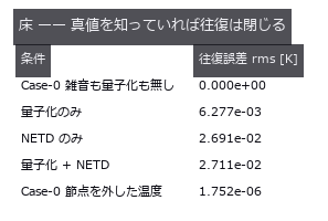
↑ The measurement ―― LWIR・350 K・ε=0.95。校正表と直接積分の相対差は最大 8.9e-16。以下の誤差はすべてこの床の上。 (figure labels are in Japanese; the numbers are the same)

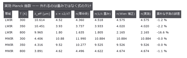
↑ n = d ln L_bb/d ln T。

↑ LWIR・T_obj = 350 K・T_refl = 300 K。

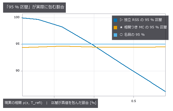
↑ 20000 試行 / 点。

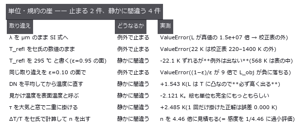
↑ 止まるのは校正表の範囲外に落ちたときだけ。

py -3.11 examples/poc_thermal_radiometry.py

Source: examples/poc_thermal_radiometry.py

This run produced 18 figures in total - see them all

Ops used (notes): beer_lambert_transmittance · interp_linear · mat_eigh · noise_sigma · photon_uncertainty · poly_fit · stat_correlation · stat_covariance · stat_describe · stat_histogram

No.2026.043 —— Depth of a Subsurface Defect by Pulsed Thermography

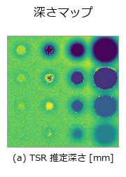
↑ Depth of a Subsurface Defect by Pulsed Thermography ―― Surface temperature after a flash, generated from the exact 1-D heat-conduction solution, with delamination depth estimated from the image sequence. Where the diameter is at least four times the depth the estimate lands within a few percent; at 0.5 mm deep and 2 mm across it is off by +627 %. The cause is not lateral diffusion but the fitting window: shortening it from 25 s to 4 s brings that case back to -9 %.

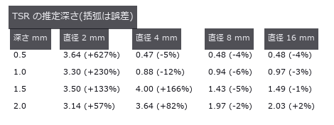
↑ The measurement ―― 右下三角(直径が深さの 4 倍以上)は数 %。左上は横拡散で壊れる。 (figure labels are in Japanese; the numbers are the same)

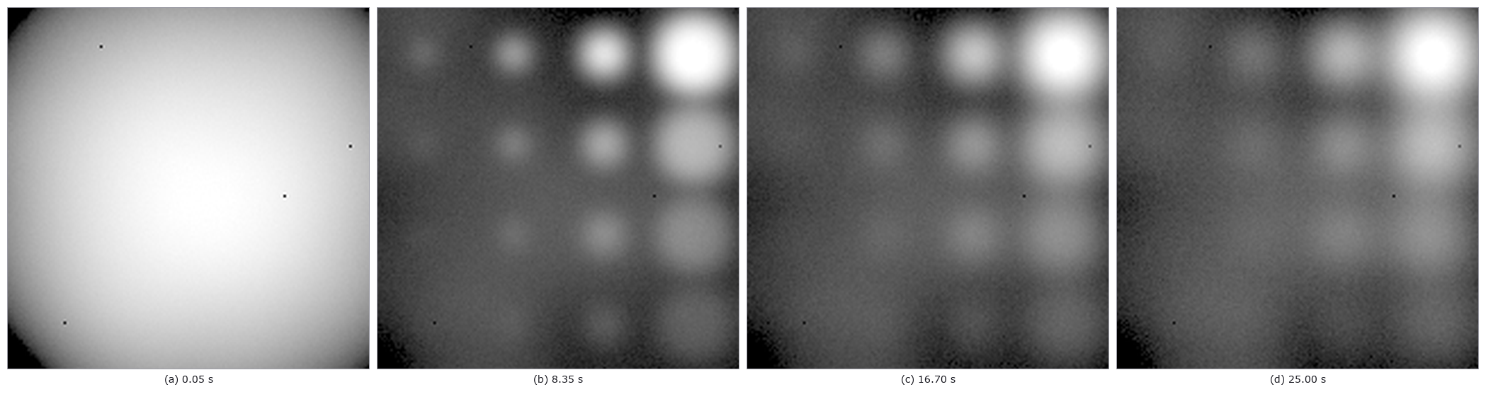
↑ Viewer-gamma grayscale; NETD 0.02 K, low-frequency NUC residual 0.08 K RMS, four dead pixels.

↑ Sequential turbo-like depth scale in millimetres; signed error at right.

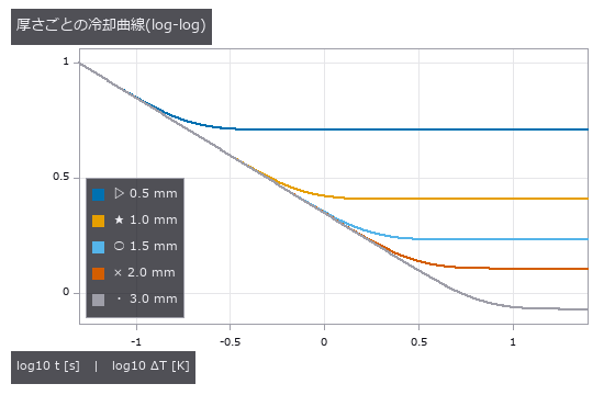
↑ 早期の勾配は -1/2。

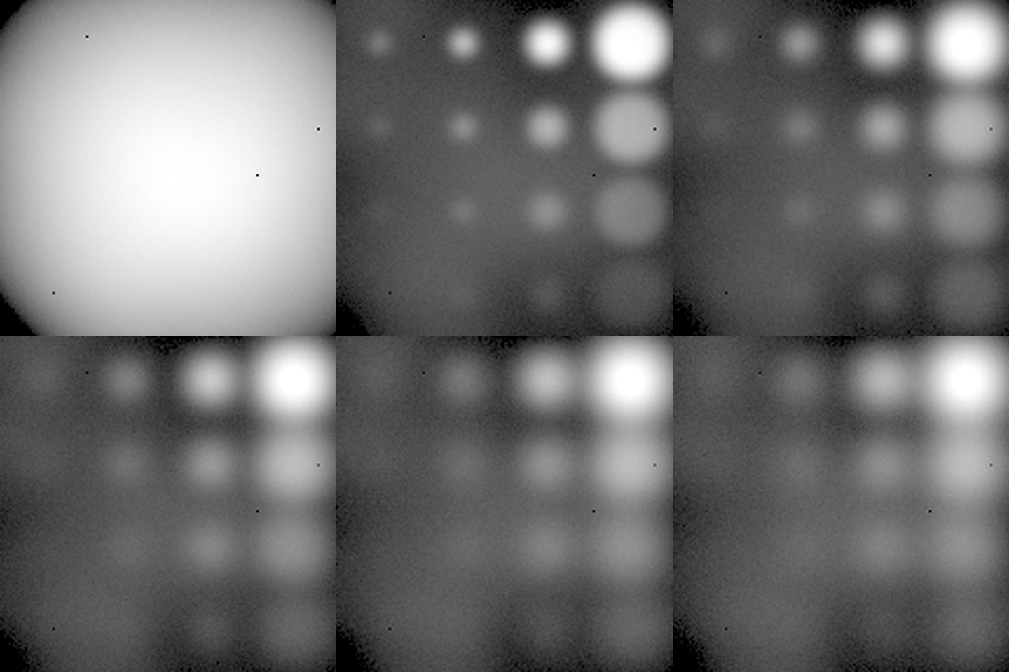
↑ The animation ―― Forty-eight uint8 cooling frames after a non-uniform flash.

py -3.11 examples/poc_thermography_ndt.py

Source: examples/poc_thermography_ndt.py

This run produced 7 figures in total - see them all

Ops used (notes): color_bar

No.2026.178 —— Measuring a Camera Without Buying One — Recovering Quantum Efficiency, Gain and Dark Noise from a Planted Sensor with the EMVA 1288 Procedure

↑ Measuring a Camera Without Buying One — Recovering Quantum Efficiency, Gain and Dark Noise from a Planted Sensor with the EMVA 1288 Procedure ―― The lead figure places 640 x 480 dark, flat and saturated frames at native scale, exposing 1 DN row, 1.5 DN column and 4 DN pixel fixed pattern plus nine planted defective pixels.

↑ The measurement ―― 平坦画像2枚の差（時間雑音）｜平坦平均−暗平均（空間雑音）｜6σ欠陥画素図。固定模様を無効化する検査では中央の空間模様が消え、ゲートは赤になる。 (figure labels are in Japanese; the numbers are the same)

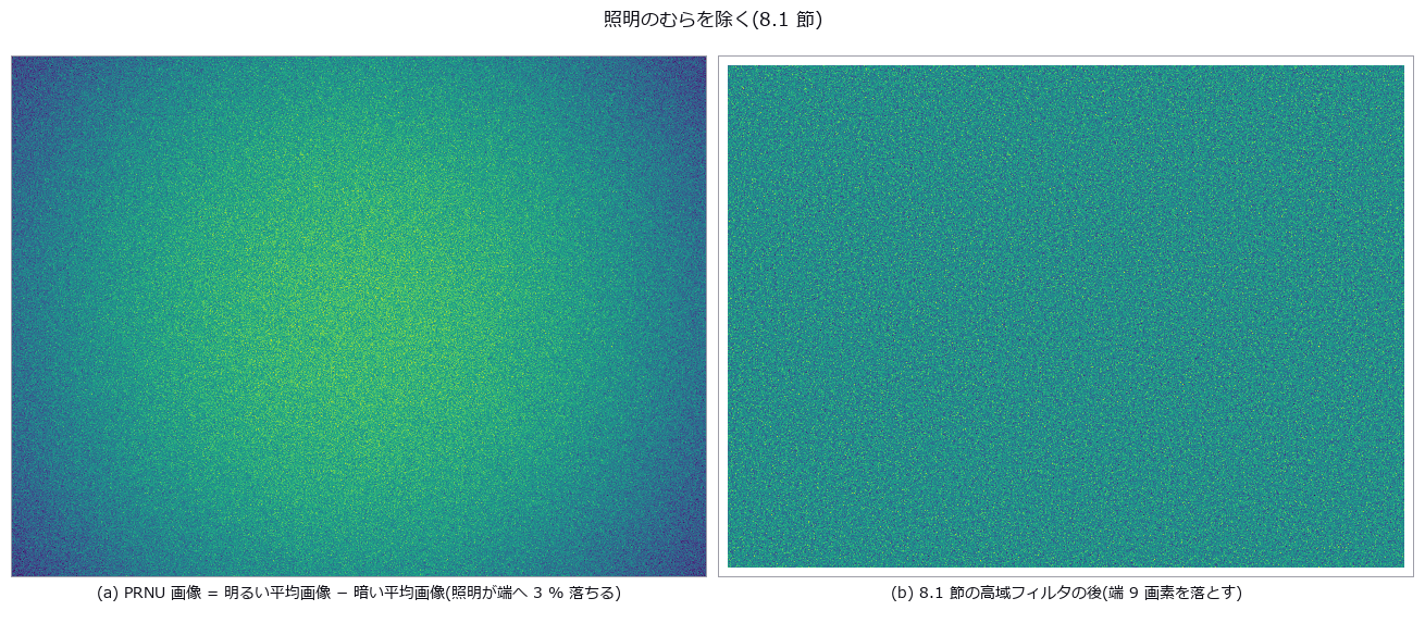
↑ 規格の模擬カメラ。

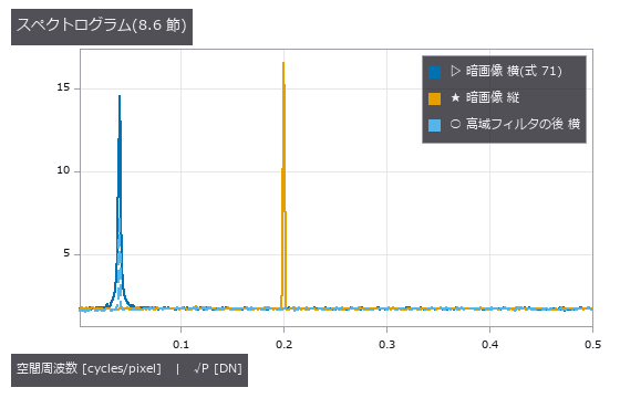
↑ 白い DSNU は平らな床(高さ = 標準偏差 1.5 DN)、正弦は鋭い山(横 0.04・縦 0.2 c/px)。

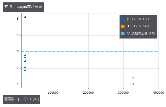
↑ 線形なセンサを乱数を変えて撮り、式 51(局所の傾きの相対偏差の平均)を出す。

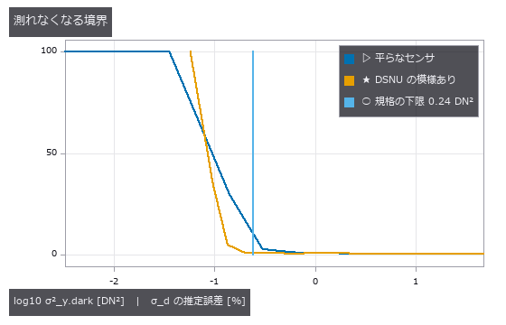
↑ 暗画像の分散が 0.24 DN² より小さいと、規格は σ_d を推定しない(式 53・54)。

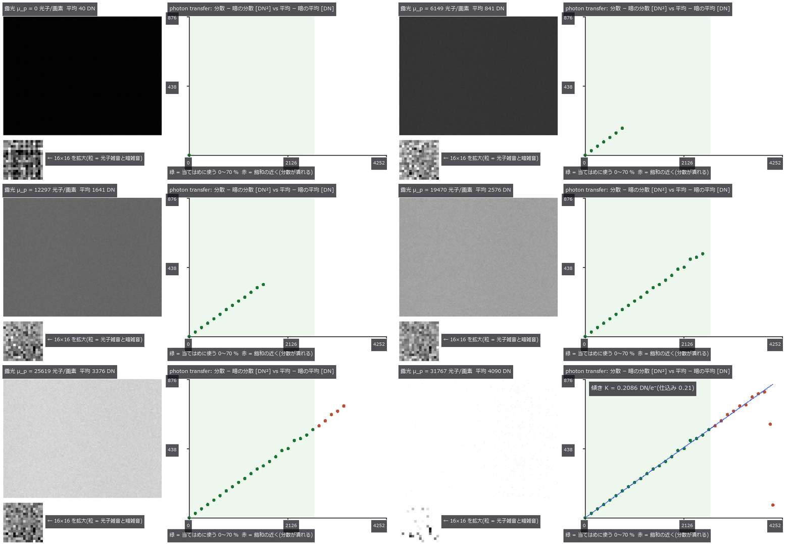
↑ The animation ―― 露光を上げながら同じ露光で 2 枚ずつ撮り、平均と時間分散(2 枚の差から、式 18)を 1 点ずつ置く。直線の傾きがシステムゲイン K = 0.2086 DN/e⁻(仕込み 0.21)。飽和の近くでは分散が潰れるので、規格は 0〜70 % の点だけで当てる。

py -3.11 examples/poc_emva1288_sensor.py

Source: examples/poc_emva1288_sensor.py

This run produced 10 figures in total - see them all

Ops used (notes): emva_dark_current · emva_defect_pixels · emva_dynamic_range · emva_exposure_for_snr · emva_highpass · emva_linearity_error · emva_pair_statistics · emva_photon_exposure · emva_photon_transfer · emva_ptc_linearity_check · emva_quantum_efficiency · emva_sensitivity_threshold · emva_snr_curve · emva_spatial_nonuniformity · emva_spectrogram · emva_total_snr · spectrogram · text_box

No.2026.090 —— Porosity in Weld Radiographs — Closing With the Share of Images Misgraded by One Class

↑ Porosity in Weld Radiographs — Closing With the Share of Images Misgraded by One Class ―― A radiograph drawn in closed form with Beer–Lambert: 10 mm plate, arc-shaped reinforcement, spherical pores, plus scatter, unsharpness and film grain. The fixed-threshold baseline counts the weld toe as pores (124 blobs, total area 15.19 mm² against 7.93 true). The detection cliff is predictable from CNR = 16.12·d²: Rose's CNR = 4 misses (0.50 mm), while the prediction that includes smoothing and the 3 px minimum area gives 0.58 mm against 0.57 mm measured. The 9 px window cap of the background-estimation op (rectangular opening) becomes a cliff: detection drops below 50 % from 2.0 mm and reaches 0 % at 2.5 mm — choosing the op chooses the measuring range. Scatter at SPR = 1 shrinks the volumetric diameter by (1+SPR)^(-1/3): -22.6 % measured against -20.6 % predicted. Images misgraded by one class: 90 % for the baseline, 23 % with the volumetric diameter.

↑ The measurement (figure labels are in Japanese; the numbers are the same)

↑ 小さい側の崖は CNR で予測どおり。

↑ 面積径は小さい側で縮む(等高線が内側)。

↑ この回の図

↑ 体積径は (1+SPR)^(-1/3) で縮む。

py -3.11 examples/poc_weld_radiograph_porosity.py

Source: examples/poc_weld_radiograph_porosity.py

This run produced 12 figures in total - see them all

Ops used (notes): blob_features · blob_label · blob_overlay · blob_select · estimate_noise · gauss_image · gen_measure_rectangle2 · gray_opening_rect · identity · log_image · measure_pairs · measure_pos · median_rect · sk_rolling_ball · xsitk_grayscale_grindpeak

No.2026.214 —— Peeling Phases One at a Time off a 2-D Powder X-ray Diffraction Image — Calibration, Azimuthal Integration, NNLS and the Unknown Phase in the Residual; References from the NIST SRM 640g Certificate and COD CIFs, with the Shared-Model Leak Measured by Deliberate Mismatch

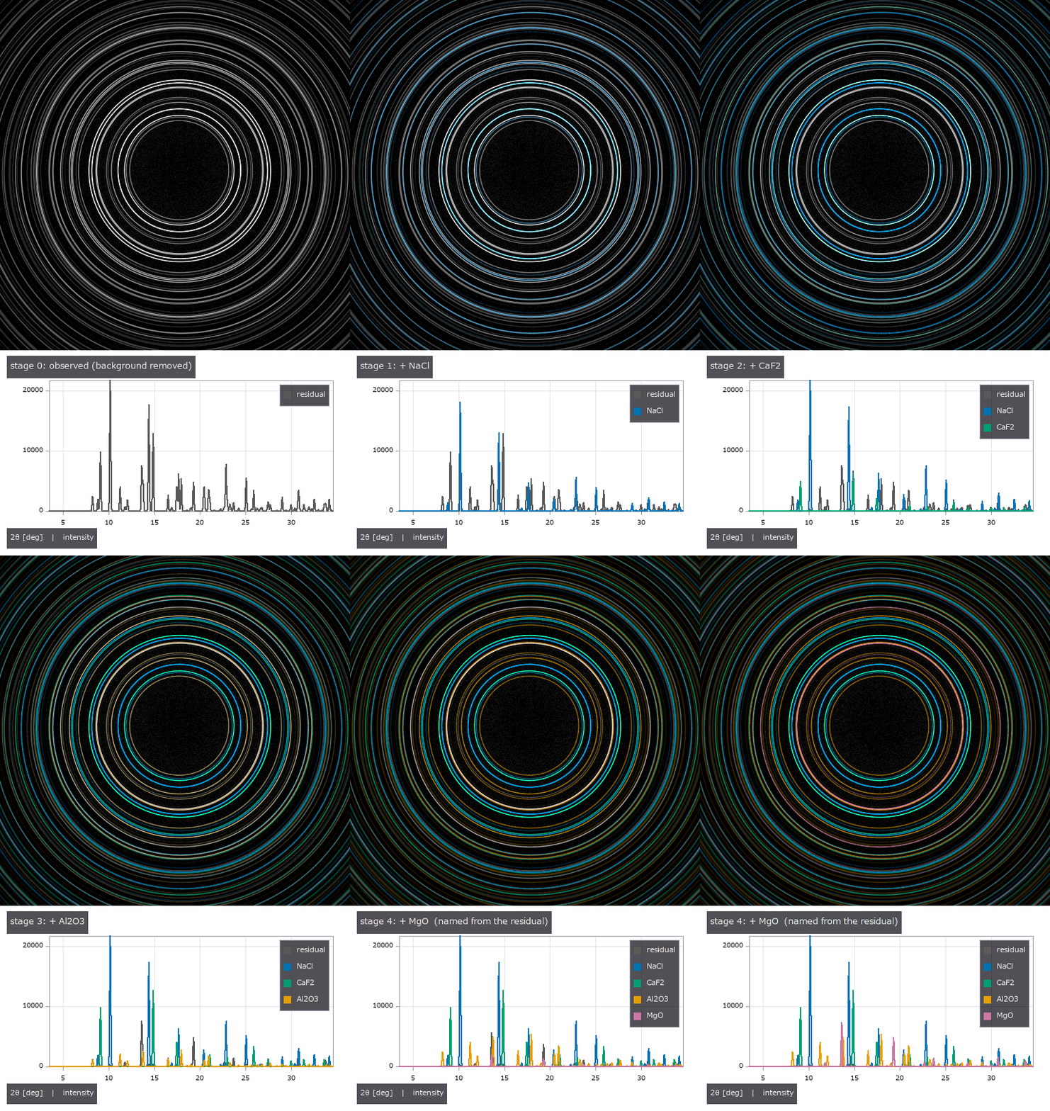
↑ Peeling Phases One at a Time off a 2-D Powder X-ray Diffraction Image — Calibration, Azimuthal Integration, NNLS and the Unknown Phase in the Residual; References from the NIST SRM 640g Certificate and COD CIFs, with the Shared-Model Leak Measured by Deliberate Mismatch ―― Shine X-rays on a powder mixture and the detector records the Debye rings of every phase on top of each other. The new module pxrd (14 ops), with no learning, calibrates the detector's centre, distance and tilt on the rings of a Si standard (at a 3° tilt: centre 0.011 px, distance 0.0009 %, tilt 3.004°, direction −40.01°, rms 0.019°), integrates azimuthally into a 2θ profile, takes the crystallite size from the peak widths by Scherrer (354 Å, truth 350 Å), peels the phases off one at a time against a reference dictionary built from CIFs (NNLS forward selection, in the order NaCl > CaF₂ > corundum, rwp 0.546 → 0.179), indexes the 8 peaks left in the residual as cubic F with a = 4.2170 Å (truth 4.2170), and names MgO among four candidates (MgO, NiO, CaO, KCl). The four-phase fractions (35 / 30 / 20 / 15 wt%) come back to within 0.04 wt%. The external reference is the NIST SRM 640g certificate: from a = 0.543 110 9 nm and Cu Kα1, Bragg plus the extinction rules reproduce its 11 tabulated lines to 0.00044° and produce no other line up to 140°. The phases are COD CIFs (CC0, kept outside the repository). Traps: integrating a 5°-tilted detector as if flat turns the rings into ellipses and splits 10 peaks into 23; a sample lattice only 0.4 % larger than the reference collapses the fractions, which return once the lattice is refined. Honestly: synthesis and analysis share one physical model, so 0.04 wt% only shows that the model's quantities survive geometry, pixels, noise and overlap. The leak was measured by deliberate mismatch: a wrong peak shape costs 0.33 wt%, ions versus neutral atoms 0.06 wt%, a crystallite size off by −29 % 0.97 wt%. Microabsorption, preferred orientation and anomalous dispersion are not in the model, and there is no external reference for intensities (measured relative intensities) yet.

↑ The measurement ―― the detector image coloured by phase (1:1 pixels, lossless PNG) (figure labels are in Japanese; the numbers are the same)

↑ the observed detector image (background removed, gamma 0.5)

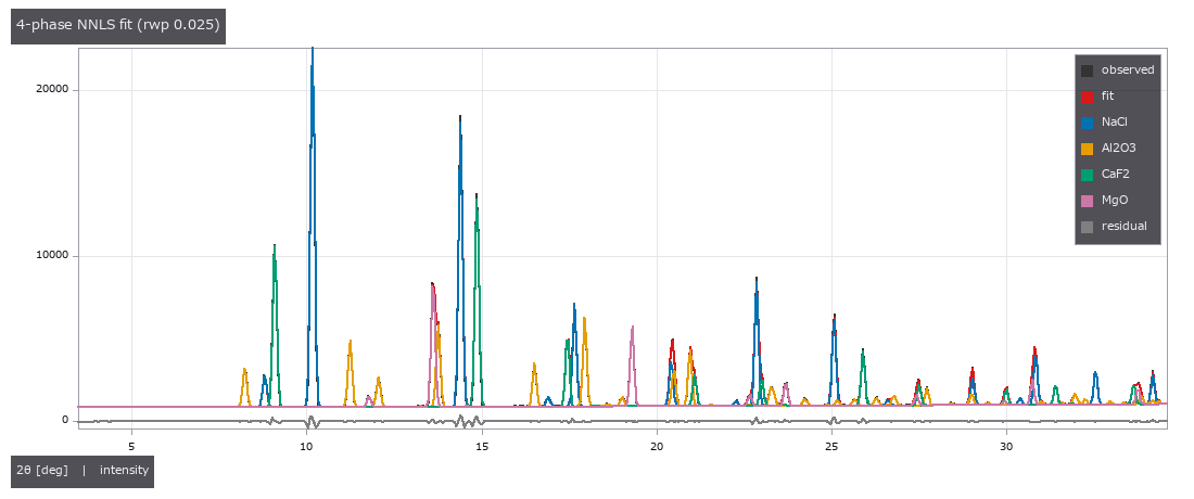
↑ integrated profile, NNLS fit and each phase's contribution

↑ この回の図

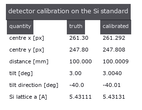
↑ この回の図

py -3.11 examples/poc_pxrd_phase_peel.py

Source: examples/poc_pxrd_phase_peel.py

This run produced 9 figures in total - see them all

Ops used (notes): axes_frame · axes_transform · azimuthal_integrate · cif_read · cubic_index · cubic_prototype · debye_ring_image · detector_calibrate · detector_two_theta · difference · diffraction_peaks · grid_lines · intensity · legend_box · nice_ticks · phase_dictionary · phase_fractions · phase_peel · plot_series · powder_reflections · scherrer_size · text_box · ticks · unexplained_peaks

No.2026.221 —— Measuring Black-Gloss and Glass from Polarisation - No Shading, but the Polarisation Remembers the Slope

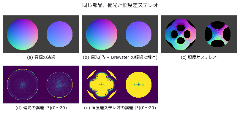
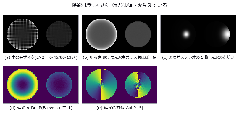
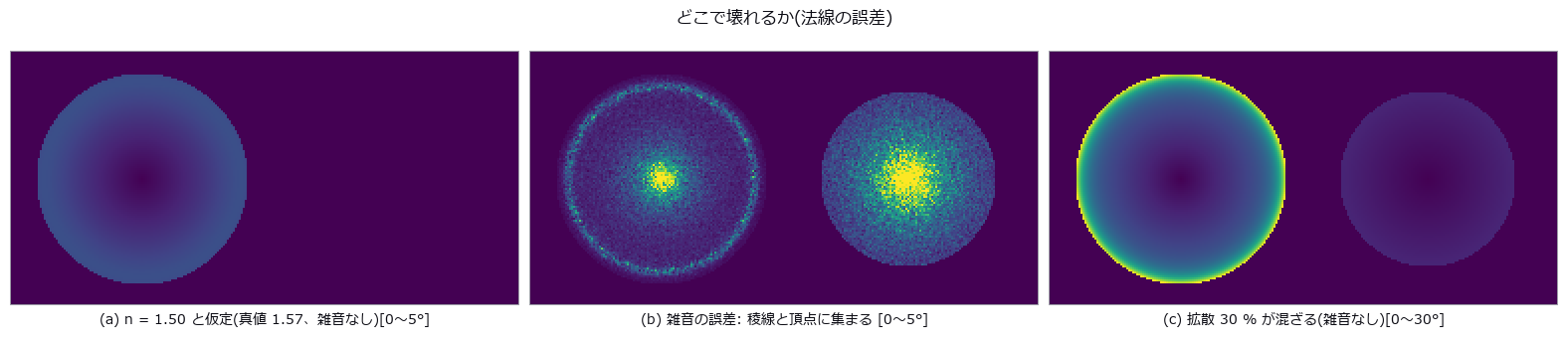
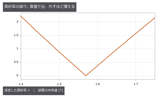
↑ Measuring Black-Gloss and Glass from Polarisation - No Shading, but the Polarisation Remembers the Slope ―― A black-glossy resin dome (n 1.57) and a glass lens (n 1.52), measured from one raw mosaic of a 4-direction on-chip polariser sensor; the truth is the analytic normals and heights used to render them. Median normal error 0.53 deg on the dome and 1.09 deg on the lens, dome height RMS 0.62 px out of 37.9 px; photometric stereo with four lights sees only the highlights on the same dome and is off by a median 26.4 deg (50x; 2,408 of 7,921 pixels get no normal at all). The ambiguity is kept: before disambiguation every pixel has four normals (two zeniths straddling Brewster's angle x the pi azimuth), the two zeniths merging on the 57.5 deg Brewster ring; convexity plus the Brewster ridge picks one. A calibration ball gives n = 1.5691 (truth 1.57) by fitting the Fresnel curve, while reading tan(theta) at the DoLP maximum gives 1.715 - a noise spike. Where it breaks: assuming n = 1.50 costs 0.89 deg and 1.40 costs 2.21 deg (exactly 0 at the truth); noise concentrates on the Brewster ring (1.27 deg) and at the apex (4.87 deg) against 0.57 deg on the flanks; 30 % diffuse light mixed in costs 7.4 deg (the two polarisations are 90 deg apart and cancel).

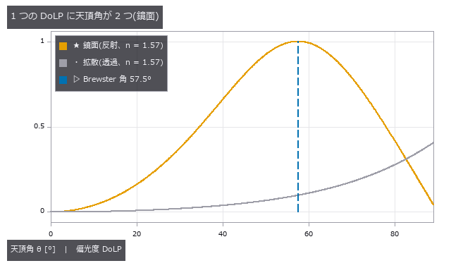
↑ The measurement ―― 鏡面の DoLP は Brewster 角でちょうど 1 になり、その両側に同じ値が 2 回出る。拡散は単調だが弱い(最大 (n²−1)/(n²+1))。 (figure labels are in Japanese; the numbers are the same)

↑ 左 = 黒光沢樹脂のドーム(n = 1.57)、右 = ガラスのレンズ(n = 1.52)。

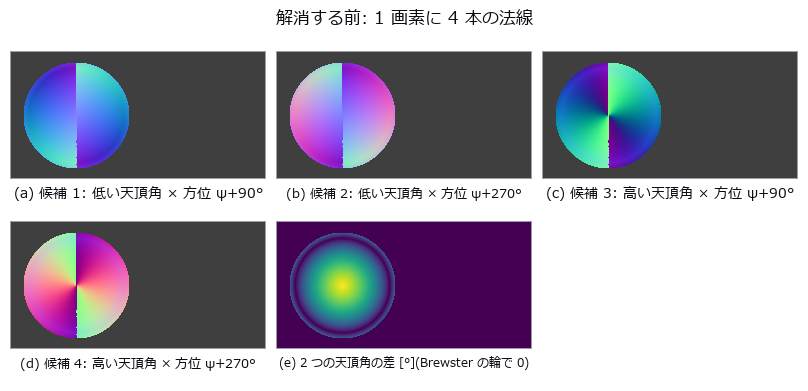
↑ 鏡面の DoLP は Brewster を挟んで 2 つの天頂角を持ち、方位は偏光子にとって π が同じ。

↑ 屈折率の誤りは全体を滑らかにずらす。

[

↑ 較正球で測れば 0.01 以内に入る([4])。

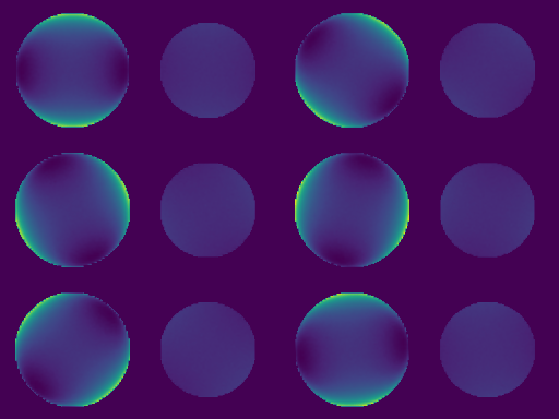
↑ The animation ―― 検光子を 0〜180° 回したときの明るさ。黒い蝶ネクタイが回る —— 暗くなる向きが、その画素の面の傾きの向き(鏡面では入射面に直交)。

py -3.11 examples/poc_shape_from_polarization.py

Source: examples/poc_shape_from_polarization.py

This run produced 10 figures in total - see them all

Ops used (notes): aolp_to_azimuth · brdf_blinn_phong · dolp_to_zenith · fresnel_dielectric · photometric_stereo_robust · polarization_demosaic · sfp_disambiguate · sfp_dolp_model · sfp_estimate_index · sfp_height · sfp_normals · sfp_render

No.2026.185 —— From Melt-Pool Thermography to X-ray CT in Metal Additive Manufacturing — Raw Signal Is Not Temperature, Time Axis and Pixel Pitch, and Powder That Clings Only to Down-Facing Surfaces

↑ From Melt-Pool Thermography to X-ray CT in Metal Additive Manufacturing — Raw Signal Is Not Temperature, Time Axis and Pixel Pitch, and Powder That Clings Only to Down-Facing Surfaces ―― In-situ thermography of metal additive manufacturing (laser powder-bed fusion, In718) linked to post-build X-ray CT with existing Fullseye ops. Real data: National Institute of Standards and Technology (NIST) open data (thermography doi:10.18434/mds2-2716; XCT doi:10.18434/mds2-2291, measured at the Georgia Institute of Technology), subsets extracted 2026-10-02 and thresholded/cropped/false-coloured here (modified; provided by NIST AS IS, https://www.nist.gov/open/license). The data is not shipped; without it the same gates run on synthetic data with ground truth. Gates: raw signal (DL) is never called temperature — conversion requires emissivity ε, the same saturated 4095 DL reads 1401 °C at ε=1 and 1641 °C at ε=0.3 (239 K apart), saturation is a lower bound, 0 means no measurement (the formula would pin it at −204 °C) / 24 laser-on segments in the scan command = 24 bursts in the thermal video, with a +2.3 % period mismatch recorded as unresolved (on synthetic data an injected 2.3 % reads back as +2.31 %) / pixel pitch from scan speed 21.31 µm (max 0.20 % across conditions) / melt-pool length varies 15× more between conditions than between repeats / CT matches the design STL cross-section at Dice 0.981, and surface protrusion is 63 µm on down-facing surfaces (hole ceilings) vs 32 µm up-facing — powder hangs only from down-facing surfaces / no internal voids (detection limit ~63 µm; the 7 enclosed air pockets all lie within 0.02 mm of the surface, trapped by stuck powder). Honestly: the calibration formula was read from an unclosed attribute string, the 1336 °C liquidus is assumed, CT voxel size is back-computed from design dimensions, and the 2.3 % time-axis mismatch is unresolved.

↑ The measurement ―― calibration T = 14388/(a ln(c eps/x + 1)) - b/a (reading of the file's model string is our assumption). 4095 DL = 1402 C at eps=1, 1641 C at eps=0.3. Pixels >= 2759 DL are above the liquidus for any eps <= 1. Source: National Institute of Standards and Technology (NIST), doi:10.18434/mds2-2716 (thermography) and doi:10.18434/mds2-2291 (XCT, measured at Georgia Tech); subsets extracted 2026-10-02, thresholded/cropped/false-coloured here (modified). Provided AS IS, https://www.nist.gov/open/license (figure labels are in Japanese; the numbers are the same)

↑ Line_0_1, row 300: 19 saturated frames are only a lower bound; the curve stops at frame 189 where the camera reports 0 (below 100 DL) instead of falli…

↑ Y pad: the command (XYPT, no time step stored) and the staring camera agree on the count and on the long last interval, yet drift apart by 2.3 % per p…

↑ slice at z = 4.00 mm just below the crown of the 4 mm hole: particles hang into the hole from the down-facing surface; red = design.

↑ XCT vs STL: protrusion = p95 of the signed distance (outward positive) after subtracting the median of each 0.25 mm surface cell (form error); line =…

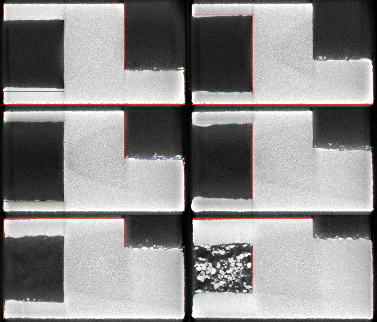
↑ The animation ―― XCT slices 121..320 (z = 1.75..4.16 mm, build direction) with the STL cross-section in red. Note the powder/dross hanging under the hole crown and the 45 deg notch. Source: National Institute of Standards and Technology (NIST), doi:10.18434/mds2-2716 (thermography) and doi:10.18434/mds2-2291 (XCT, measured at Georgia Tech); subsets extracted 2026-10-02, thresholded/cropped/false-coloured here (modified). Provided AS IS, https://www.nist.gov/open/license

py -3.11 examples/poc_am_thermal_to_ct.py

Source: examples/poc_am_thermal_to_ct.py

This run produced 9 figures in total - see them all

Ops used (notes): blob_features · blob_label · blob_select_largest · median · mesh_slice_stack · seg_boundary_f · seg_dice_jaccard · signed_surface_distance · sk_otsu · vol_boundary_points · vol_gaussian · vol_label · vol_region_props

No.2026.225 —— How Much the Bright SEM Edge Inflates a Dimension — the Shape Matches but the Area Grows

↑ How Much the Bright SEM Edge Inflates a Dimension — the Shape Matches but the Area Grows ―― The lead figure puts two electron-image contrasts side by side and overlays truth, detections and edge bias. Ten times the dose gives 3.16x SNR; edge-area bias grows toward small defects.

↑ The measurement ―― 0.5 nm/pixel で再計算した 256 nm 視野。明帯幅は PSF とともに増える。 (figure labels are in Japanese; the numbers are the same)

↑ 低照射量ほど粒状のショット雑音が増える。

↑ 合成 SEM 像(半径 22 px の円錐欠陥、PSF σ=3)。

↑ 面積の太りは小さい欠陥ほど大きい(周囲長/面積 ∝ 1/R)。

py -3.11 examples/poc_sem_wafer_defect_edge_bias.py

Source: examples/poc_sem_wafer_defect_edge_bias.py

This run produced 5 figures in total - see them all

Ops used (notes): blob_features · blob_label · pod_hitmiss_fit · seg_boundary_f · seg_dice_jaccard · sem_image · sem_render

No.2026.228 —— A Pseudo-Simulation of a Gravitational-Wave Detector — Cavity Optics, the Quantum-Noise Budget and the Matched Filter in Closed Form, Scored on the Real GW150914 Data

↑ A Pseudo-Simulation of a Gravitational-Wave Detector — Cavity Optics, the Quantum-Noise Budget and the Matched Filter in Closed Form, Scored on the Real GW150914 Data ―― How much of a km-scale Michelson interferometer reading a strain of 1e-21 can be reproduced in closed form, scored on the public GW150914 data (GWOSC) and the published numbers. Twelve new ops: the arm cavity (fabry_perot_response gives finesse 445 and a 42 Hz pole from the public aLIGO design values, cavity_strain_transfer, michelson_dc_readout, pdh_error_signal with the slope of Black 2001 to 0.9999), the quantum-noise budget (quantum_noise_budget: shot x radiation pressure = SQL^2/2 as an identity, and the second implementation gwinc 0.6.2 agrees within 0.96 to 1.12 at eight frequencies) and the signal side (psd_welch -> whiten_by_psd -> matched_filter_snr / optimal_snr, chirp_newtonian, chirp_mass_from_track, coincidence_delay). On the real data, whitening plus a 35-350 Hz band correlates at 0.959 / 0.935 with the published Fig. 1 of PRL 116, 061102; the matched filter with the numerical-relativity waveform gives SNR 19.0 (H1) / 13.1 (L1) against the published ~20 / 13, a network SNR of 23.1 against 24, and L1 leading by 7.1 ms against 6.9 ms. The Newtonian chirp reaches only 9.1 / 5.6 (no merger or ringdown). The ratio to the design curve (T1800044) is 0.42 at 20 Hz, 1.99 at 100 Hz and 0.33 at 1 kHz, which the table attributes to signal recycling and thermal noise. The take-home for inspection: a known waveform in 1/f^2 coloured noise is recovered by the whitened matched filter at the injected height, while plain correlation keeps 0.98 for a narrowband tone but only 0.50 for a chirp and 0.37 for a ring-down. The real-data stage runs when the files are placed and says 'not placed' otherwise. Nothing is learned, nothing is calibrated.

↑ The measurement ―― 単極 1/√(1+(f/f_p)²) × 往復伝搬の sinc(2πfL/c)。極で 1/√2、FSR = c/2L で零。 (figure labels are in Japanese; the numbers are the same)

↑ 反対称で共振で零。

↑ 通常干渉計(信号再利用なし)の量子雑音。

↑ 数値相対論の波形は公表どおりの山を立て、ニュートン近似(合体・リングダウン無し)は半分以下。

↑ 雑音が 1/f² のとき、波形が低周波を含むほど素の相関は損をし、白色化した整合フィルタは最適 SNR どおりに拾う。

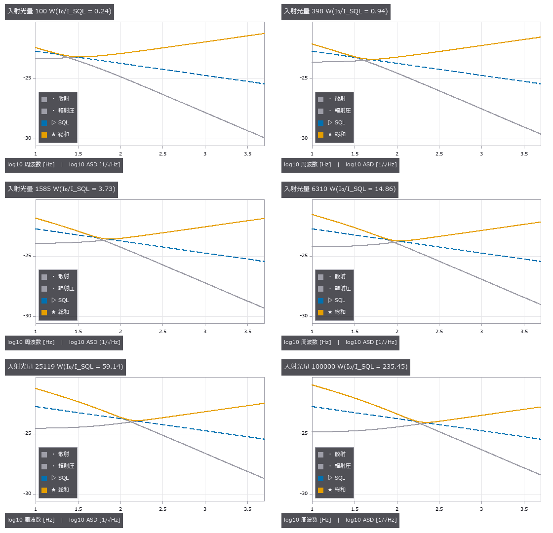
↑ The animation ―― 入射光量 100 W → 100 kW: 散射雑音は 1/√P で下がり、輻射圧雑音は √P で上がる。総和は K = 1 の周波数で SQL に触れ、その点が光量とともに高い周波数へ動く。

FULLSEYE_GWOSC_DATA=<dir> py -3.11 examples/poc_gw_detector_pseudo_simulation.py

Source: examples/poc_gw_detector_pseudo_simulation.py

This run produced 7 figures in total - see them all

Ops used (notes): bandpass · cavity_strain_transfer · chirp_mass_from_track · chirp_newtonian · coincidence_delay · fabry_perot_response · matched_filter_snr · michelson_dc_readout · optimal_snr · pdh_error_signal · psd_welch · quantum_noise_budget · spectrogram · whiten_by_psd

No.2026.234 —— Finding Micrometre Dents a Photograph Cannot Show, in the Mirror Image of a Fringe Screen — Phase-Measuring Deflectometry

↑ Finding Micrometre Dents a Photograph Cannot Show, in the Mirror Image of a Fringe Screen — Phase-Measuring Deflectometry ―― A dent a few micrometres deep in a glossy surface (a painted car panel, a cover glass) is all but invisible in a lit photograph, because a mirror only shows the light. Put a screen in front of the surface, show phase-shifted fringes and photograph their mirror image: a tilt of 1e-3 rad moves the reflected point 0.6 mm on a screen 30 cm away. Six new ops (deflectometry, category deflectometry of opsspecular): the rig, the screen pattern, the forward render (height field to fringe mirror image, with a diffuse fraction, scatter, the back reflection of glass, aperture-integrated focus and noise), phase to normals (via match3d.normal_from_reflection), slope to curvature (one derivative, no integration) and the closed-form sensitivity. On a painted panel with 3 µm and 1 µm dents, 0.8 µm waviness and 0.12 µm polishing marks the photograph's defect signal peaks at 0.00066 (0.17 of one 8-bit step) while the curvature map shows the dents at SNR 110 and 57, and the integrated depth is within 0.5 % of the truth. Phase noise matches sqrt(2/N) sigma/b at 1.00 and slope noise is 0.67 of sigma_u/(2d), the sqrt(4/9) of bilinear resampling. Where it breaks: lifting the part by 0.3 mm adds the apparent tilt dz sin(theta)/d (to 0.1 %) and a 388 m bowl while the dent depth moves 0.7 %; a 2 % screen-distance error makes dents 2.3 % shallower; a 1 µm dent survives a diffuse fraction of 0.85 and fringe orders start to jump at 0.9; on uncoated cover glass the back-surface light is bent the other way by the dent's wedge, so the slope sensitivity shrinks to the closed-form 0.246 (measured 0.246) and dents look a quarter as deep; with an 8 mm aperture, focusing on the surface leaves 0.60 of the fringe amplitude and focusing on the screen leaves 0.52 of the depth. Nothing learned, nothing calibrated, 22 gates.

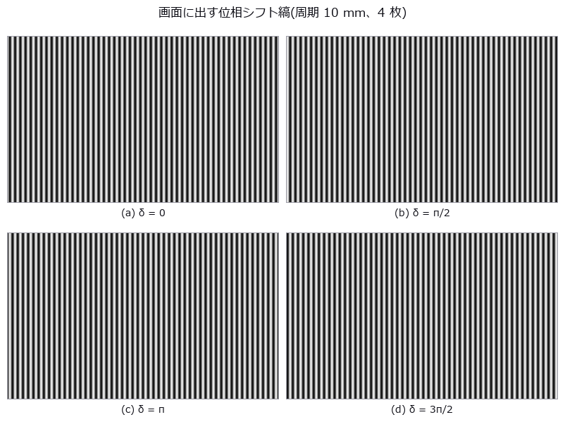
↑ The measurement ―― 面の前の画面(520 × 320 mm)にこの 4 枚を順に出し、面に映った鏡像を撮る。縦縞は画面の u(入射面内)を、同じ 4 枚を横縞にしたものが v を符号化する。粗い縞(周期 160 mm)の 4 枚で次数を決める。 (figure labels are in Japanese; the numbers are the same)

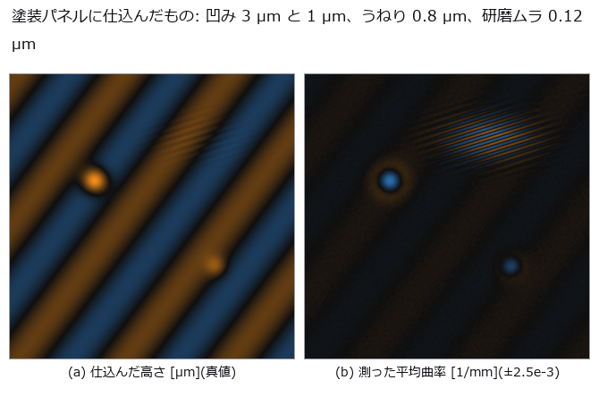
↑ 左が真値の高さ(視野 40 mm、青 = 高い・橙 = 低い)。

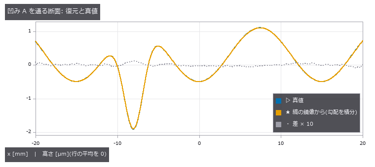
↑ 真値(破線)と復元(実線)はほぼ重なるので、差を 10 倍にして点線で重ねた。

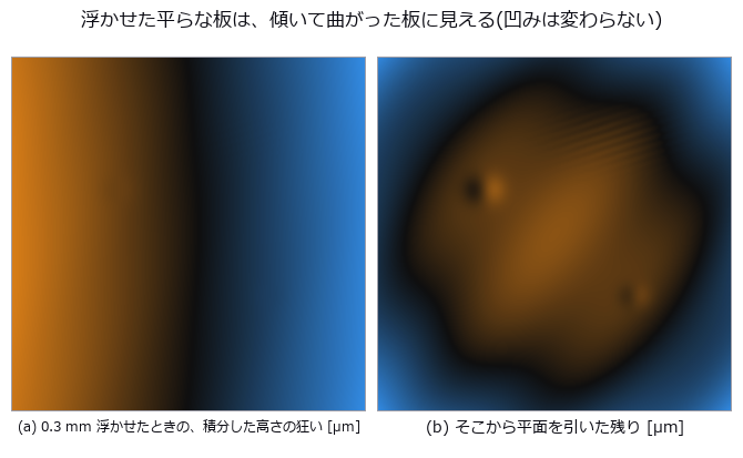
↑ 平らな板を 0.3 mm 浮かせただけで、測った高さは 40 mm で約 14 µm 傾く(左、視野の中心で 3.4e-4 rad)。

↑ 表と裏の反射率はほぼ同じ(R1 0.043、R2 0.039)なので、2 つの縞の和の位相は上限 1.16 rad までずれ得る。

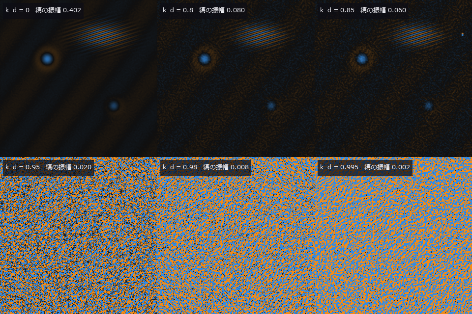
↑ The animation ―― 拡散成分 k_d = 0, 0.5, 0.8, 0.85, 0.9, 0.95, 0.98, 0.99, 0.995 と上げていったときの平均曲率(±2.5e-3 /mm)。雑音が 1/(1 − k_d) で増え、浅い凹み B が先に沈み、最後は粗い縞の次数が飛ぶ。

py -3.11 examples/poc_phase_measuring_deflectometry.py

Source: examples/poc_phase_measuring_deflectometry.py

This run produced 14 figures in total - see them all

Ops used (notes): absolute_phase · deflectometry_phase_to_slope · deflectometry_render · deflectometry_rig · deflectometry_screen_pattern · deflectometry_sensitivity · fresnel_dielectric · integrate · sfp_height · slope_to_curvature · text_box · wrapped_phase

No.2026.235 —— TDI Line Scan and Line-Scan Lenses — Stages Reveal the Defects, a Sync Error Smears Them, and a C-Mount Lens Loses the Ends of a Long Sensor

↑ TDI Line Scan and Line-Scan Lenses — Stages Reveal the Defects, a Sync Error Smears Them, and a C-Mount Lens Loses the Ends of a Long Sensor ―― Moving material (film, steel strip, wafers) is imaged with line sensors, and on a dark line TDI adds N stages of exposure. Six new ops (linescan, category linescan of opsoptics): TDI SNR from the EMVA 1288 linear model (charge-domain and digital summation), the closed-form MTF of a synchronisation error and of yaw, an acquisition that transports a reflectance map past the sensor (speed error, yaw, weave, encoder sync, lens, noise), a ray-traced profile of illumination and MTF across the image height, per-column lens maps and two example lenses. On a dark cold-rolled steel strip at 40 photons per stage, the SNR measured from the temporal noise of image pairs matches equation 21 within 1.2 % at every stage count. Digital summation gains exactly √N (×8.09 at 64 stages), charge summation pays the read noise once and gains ×26.9. Detection of a faint scratch, pinholes and an inclusion goes from 0 of 3 at one stage to 3 of 3 at 64 stages with no false alarms. A speed error ε smears the image by N·ε pixels and the scan MTF follows |sinc(f N ε)|, printed first and then measured on a sine chart: largest difference 0.0035 over 45 conditions. A ±3 % speed ripple drops the local MTF to 0.64 when free-running and is fully removed by encoder sync; the cross-direction blur of yaw, |sinc(f N sin θ)|, is not (largest difference 0.0017). The same triplet optimised for a 57 mm line (f 90) and for a 2/3-inch format (f 35, a C-mount lens reused) was ray-traced: illumination splits exactly into cos⁴ × pupil × distortion (2e-16), the line-scan lens keeps 0.976 at the end of the sensor (cos⁴ alone gives 0.855; barrel distortion of −2.9 % adds ×1.111), and the C-mount lens delivers no light beyond 19.7 mm. Flat-field correction evens the brightness (0.961 to 1.000) but leaves the sine modulation unchanged (difference 0.0006), and the CNR of an inclusion at 14 mm stays at 1.52 to 1.54 with the C-mount lens against 2.49 with the line-scan lens. Nothing learned, nothing calibrated, 19 gates.

↑ The measurement ―― EMVA 1288 の 2 枚撮り(時間雑音)で測った SNR と、式 21 を段数倍した閉形式。 (figure labels are in Japanese; the numbers are the same)

↑ ε は搬送速度とラインレートの相対誤差。

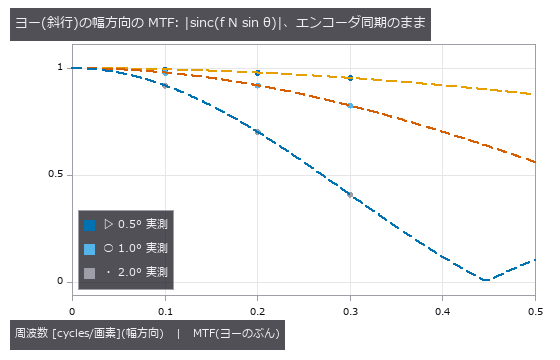
↑ web が走査軸から θ 傾くと、64 段の間に幅方向へ 64·sin θ 画素ずれる。

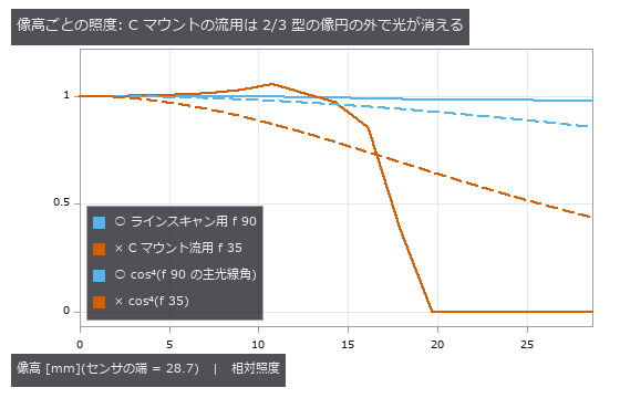
↑ 光線追跡(射影立体角の一様格子)で数えた照度。

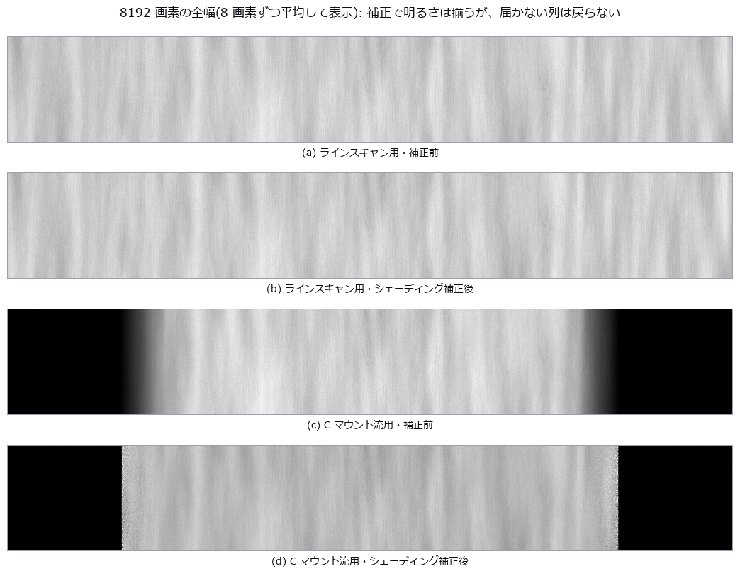
↑ 同じ明るさの尺度で表示。

py -3.11 examples/poc_tdi_linescan.py

Source: examples/poc_tdi_linescan.py

This run produced 10 figures in total - see them all

Ops used (notes): emva_pair_statistics · lens_field_profile · lens_shading_correct · lens_shading_gain · lens_system · linescan_acquire · linescan_lens_columns · linescan_lens_example · paraxial_trace · relative_illumination · tdi_snr · tdi_sync_mtf

No.2026.236 —— Pixel-Shift Imaging — Shift the Sensor One Pixel and False Colour Vanishes, Half a Pixel and Aliasing Vanishes; the MTF Does Not Rise

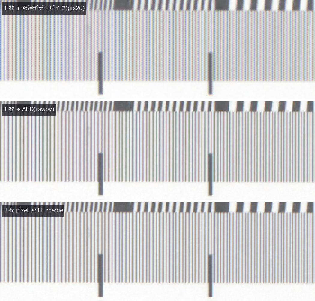
↑ Pixel-Shift Imaging — Shift the Sensor One Pixel and False Colour Vanishes, Half a Pixel and Aliasing Vanishes; the MTF Does Not Rise ―― The lead chapter runs on real raw data: four pixel-shift frames from a 35 mm full-frame mirrorless camera with sensor shift (PixelShift200, Qian et al., ICCP 2022, CC BY 4.0) of a resolution chart. The camera cycles (0,0)→(1,0)→(1,−1)→(0,−1); passing the op's default order flags 23.2 % of the static scene as moving (0.09 % with the right order). The merge matches the authors' own merged RGGB to a correlation of 0.99999996, false colour on the achromatic chart drops from 0.054 (single frame, bilinear) to 0.025, and bars finer than 0.25 cyc/px keep 1.67 times the contrast; a good demosaic (AHD in rawpy) comes within 1 % of the four-frame contrast with 0.020 colour, because the chart's finest bars stop at 0.31 cyc/px. The synthetic chapters that follow sweep the failure conditions. What pixel shift (moving the sensor by one or half a pixel with a piezo actuator) adds to visual inspection and what it does not. Six new ops (pixelshift, category pixelshift of opsoptics): shift sequences with actuator error, an exact box-aperture capture through a shifted Bayer or monochrome sensor, a grid merge with the nominal shifts that refuses sequences that cannot fill the grid, a motion mask, a false-colour metric and the closed-form budget (sinc times diffraction MTF, Q = λN/p). Four 1-pixel shifts take false colour from 0.043-0.084 to zero on PCB traces, cloth, halftone print and a resolution chart (zero by construction when static and exact: R, G and B at every pixel see the same point through the same aperture). Half-pixel shifts move the FFT peak of 0.6-0.9 cyc/px gratings from the alias 1 − f₀ back to f₀, with heights matching 0.4·sinc(f₀) to 2e-14. The slanted-edge MTF50 is 0.478 single, 0.475 shifted and 0.467 cyc/px closed form: shifting removes aliasing, not MTF loss. Drizzle, an independent implementation, puts the peak at 0.700, and at 0.300 if handed the sensor shifts unchanged, because its sign convention is the opposite. With 3.45 µm pixels and f/1.4 to f/22 the 0.7 cyc/px modulation follows sinc times the diffraction MTF to 0.0008, vanishes beyond Q = 1.43, and the resolution gain ends at Q = 1.47, before the aliasing boundary Q = 2. A 0.5 fill factor gives 3.2 times the modulation at 0.8 cyc/px. Failure modes: a single frame off by 0.05 px gives the colour error 2πf·a·sinc·δ/√2 to 1.2 %; random error of 0.1 px gives false colour 0.012 against 0.053 for a single demosaic. A moving part at 0.25 px per frame still beats a single demosaic (0.161 against 0.205), but from 0.5 px per frame the merge is worse; falling back to one frame where the greens disagree reaches the single-frame ceiling with no false detections on static areas. Noise falls as σ/√c for R and B and σ/√(2c) for G within 2.1 %, but on a moving grating more frames mean more error (0.081 to 0.273 from 4 to 16 frames). Nothing learned, nothing calibrated, 34 gates.*

↑ The measurement ―― 基板の配線・織物・網点・解像チャート(上から)。左 = 3 色を各画素で取る理想センサ、中 = Bayer 1 枚 + 双線形デモザイク、右 = 1 画素シフト 4 枚。44 × 44 画素を最近傍で 5 倍。静止・誤差 0 では 4 枚の偽色は定義上 0(4・5 章が壊れる条件)。 (figure labels are in Japanese; the numbers are the same)

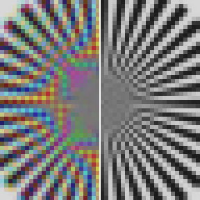
↑ 解像チャートの 星形チャート(48 × 48 画素を 6 倍)。

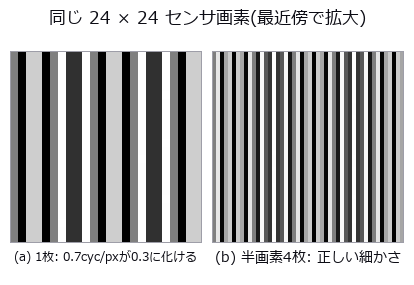
↑ 左は画素 1 つ = 8 × 8、右は出力画素 1 つ(= ½ センサ画素)= 4 × 4 で表示。

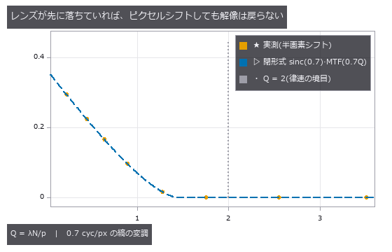
↑ 画素 3.45 µm、λ 0.55 µm で F 1.4〜22。

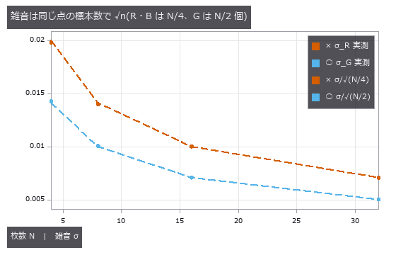
↑ 4 枚のピクセルシフトは雑音を下げるためのものではない(R・B は 1 枚と同じ)。

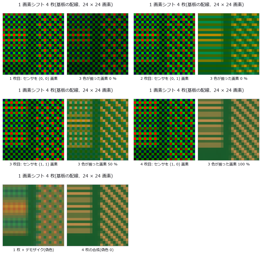
↑ The animation ―― 左 = その枚の Bayer の生の値(画素ごとにフィルタの色で表示、センサの位置へずらして描く)、右 = 合わせた格子に R・G・B が揃っていく様子。最後は 1 枚のデモザイクと 4 枚の合成(24 × 24 画素を 10 倍)。

py -3.11 examples/poc_pixel_shift.py

Source: examples/poc_pixel_shift.py

This run produced 15 figures in total - see them all

Ops used (notes): airy_pattern · annotate_figure_grid · drizzle_resample · edge_spread · false_color_metric · halftone_screen · mtf50 · mtf_diffraction · pixel_shift_capture · pixel_shift_merge · pixel_shift_motion_mask · pixel_shift_pattern · pixel_shift_resolution_budget · psnr · raw_demosaic_bilinear · reflect · sfr_from_edge · text_box · weave_normals

No.2026.243 —— Indirect Time of Flight, Multi-Frequency — Higher Frequencies Measure Finer, but Wrapping, Multipath, Flying Pixels and Harmonics Break It

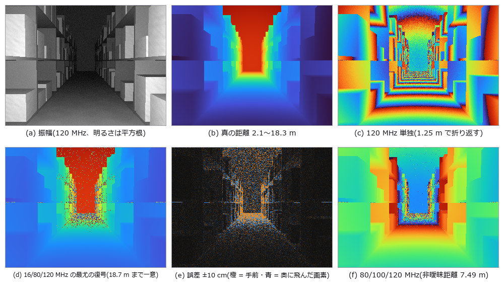
↑ Indirect Time of Flight, Multi-Frequency — Higher Frequencies Measure Finer, but Wrapping, Multipath, Flying Pixels and Harmonics Break It ―― Continuous-wave indirect time of flight (modulated light, correlation sampled at four phase steps) taken from raw buckets to depth and into its failure modes. Eight new ops (itof, category itof of opsoptics): a capture model with shot noise, ambient light, extra paths and pixel-aperture mixing; phase, amplitude and offset; the closed-form noise budget; multi-frequency unwrapping by exhaustive maximum-likelihood hypotheses, residue_crt or the two-frequency beat; a wrong-order probability bound; two-path separation by matrix pencil; a flying-pixel mask; and cyclic-error correction. Depth noise matches c/(4πf)·√((B+σ_r²)/2)/A to 0.999-1.029 over 11 conditions with SNR ≥ 3, and Lange's formula exactly. 16/80/120 MHz is unambiguous to 18.7 m; the wrong-order rate is 0.116 at σ_φ = 0.33 rad (union bound 0.132). On the same raw signal residue_crt gives 0.1161, on par with maximum likelihood, because it now picks its anchor the Wang-Xia way (the band with the smallest noise variance); anchoring on 16 MHz, as before the fix, gave 0.556. With 80/100/120 MHz, shelves beyond 7.5 m silently fold to near range. A box under packaging film is pulled forward at one frequency (matching tof_multipath_phase); an 8-frequency matrix pencil (20-160 MHz) recovers every pixel to 2 cm at 0.8 m separation but nothing at 0.2 m or less. A room corner reads 8-99 mm too far everywhere, matching the one-bounce transport to 1e-15 m. The mask flags 97 % of the pixels floating off box edges and removes 0.03 % of step-free pixels. The ±84.8 mm square-wave cyclic error matches atan(u/(1−u)) and inverts to the 2.1 mm noise floor. Sunlight at 50 times the signal raises far wrong-order errors from 12 % to 93 %. Direct ToF on the same tabletop neither floats edges nor shifts under the film. On public raw sensor data (3 frequencies × 3 steps; Lawin, Forssén, Ovrén, ECCV 2016; Zenodo; CC BY 4.0) jumps over 30 cm are 0.131 for maximum likelihood and 0.131 for residue_crt (10-frame average; 0.293 before the anchor fix); discarding low-margin pixels keeps 68 % at 0.020. Nothing learned; calibrated only by 16 rail points and the left half of the real data; 30 gates.

↑ The measurement ―― 平らな板(距離は一様乱数)で信号を振り、次数を誤った画素の割合を数えた。破線は候補ごとのガウスの 2 仮説の誤りの和(和集合の上界)、点線はその最大の 1 項。実測は 2 本の間に入る。 (figure labels are in Japanese; the numbers are the same)

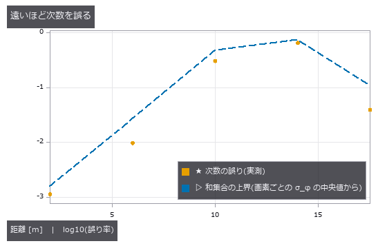
↑ 通路の画素を距離帯に分け、次数を誤った割合と、その帯の位相雑音から見積もった上界を並べた。

↑ 向かいの壁で 1 回以上反射した光が遅れて混ざり、内角の面は全体に奥へ伸びる。

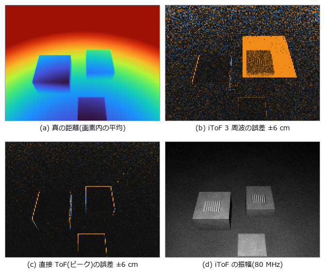
↑ 同じ卓上の場面を 2 つの方式で撮る。

↑ σ_d = c/(4πf)·√((B + σ_r²)/2)/A。

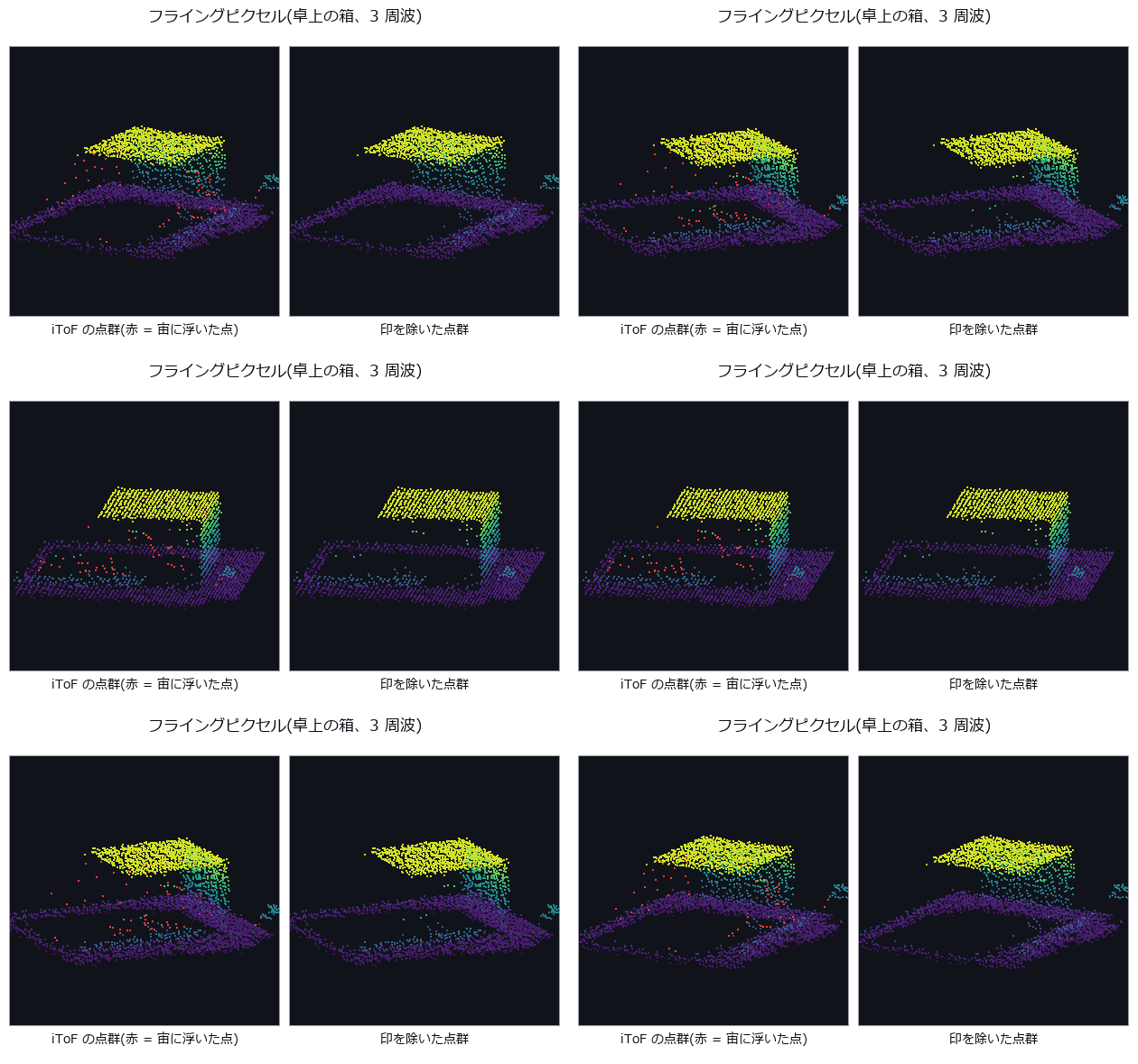
↑ The animation ―― 左の箱の点群を回して見る。横から見ると、縁から背後の床へ視線に沿って伸びる赤い点の列(フライングピクセル)が現れる。右は印を除いたもの。

py -3.11 examples/poc_itof_multifreq.py

Source: examples/poc_itof_multifreq.py

This run produced 14 figures in total - see them all

Ops used (notes): annotate_figure_grid · camera_rays · dtof_cube_depth · dtof_cube_simulate · erfc · form_factors_2d · gamma · gaussian · groove_profile · itof_capture · itof_flying_pixel_mask · itof_multipath_separate · itof_noise_budget · itof_phase_amplitude · itof_unwrap_error_rate · itof_unwrap_multifreq · itof_wiggling_correct · residue_crt · tof_multipath_phase · tof_transport_depth · transport_matrix_radiosity

No.2026.241 —— Industrial OCT — Layer Thickness and Hidden Defects of Paints, Coatings and Multilayer Films, Seen in Depth by the FFT of One Spectral Interferogram

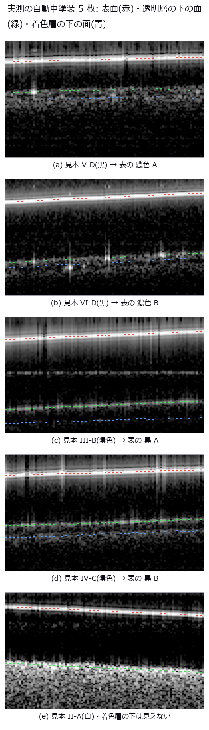
↑ Industrial OCT — Layer Thickness and Hidden Defects of Paints, Coatings and Multilayer Films, Seen in Depth by the FFT of One Spectral Interferogram ―― Optical coherence tomography sees the layer stack of paints, conformal coatings, adhesive layers and multilayer films, and voids and delaminations inside them, without cutting. Thirteen new ops (octscan, category oct of opsoptics): closed-form design numbers before measuring, interferogram simulators driven by the material table, k-linearisation, dispersion compensation and estimation, A- and B-scans, layer thickness through the group index (refusing layers that cannot be separated), boundary tracing, surface flattening and an entry point for raw spectra. Real data: public raw spectra of automotive paint panels (CC BY 4.0) processed with Fullseye ops alone give clear-coat thicknesses within 1.5 µm of the paper's OCT and 3.6 µm of the microscope, base coats within 2.3 µm of the microscope for three of four panels (one is 7.6 µm off and unresolved), a refusal under the white base coat, and an autocorrelation ghost lying flat at the clear coat's optical thickness. Synthetic: thickness through the group index within 0.04 µm of the truth, SNR, roll-off and dispersion broadening matching the closed forms, refusal below 1.4 point-spread widths, a coating-thickness map and void/delamination detection.

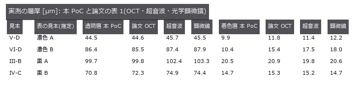
↑ The measurement ―― 屈折率は論文と同じ 1.56(透明層)・1.64(着色層)。表のどの行がどのファイルかは論文に無く、透明層の厚さで決めた(推定)。着色層はその対応と独立の突き合わせ。 (figure labels are in Japanese; the numbers are the same)

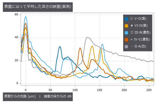
↑ 黒・濃色は透明層の下の面と着色層の下の面の 2 つの山。

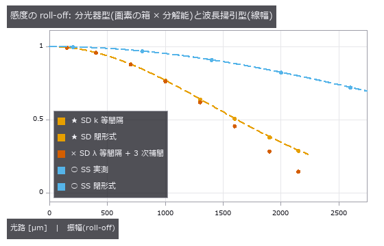
↑ SD 840/50 nm 2048 画素(深さ範囲 2.26 mm)、SS 1310/100 nm・瞬時線幅 0.1 nm。

↑ 試料腕が参照光と同じ桁に強いと、層の上下の面どうしの干渉が 0 の近くに立つ。

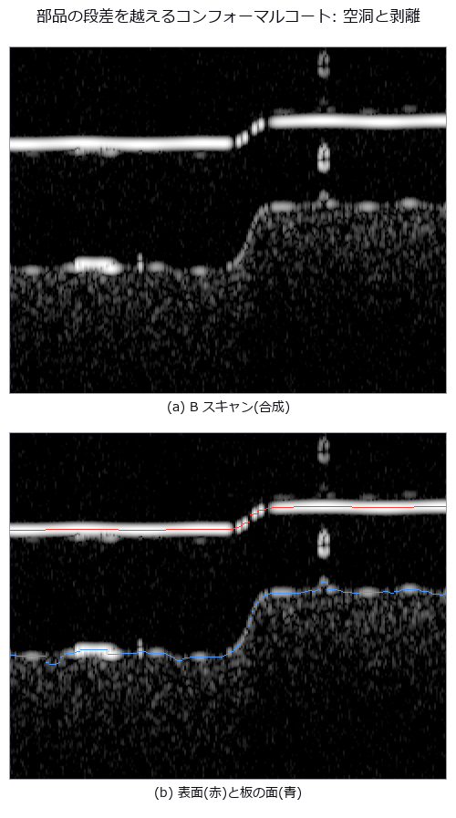
↑ 横 1.2 mm、縦は光路 25〜440 µm。

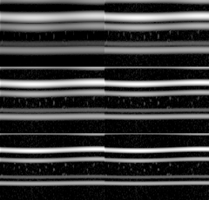
↑ The animation ―― 試料腕に溶融石英 12 mm の分散の不一致。補償の係数 a2 を 0 から 35.6 µm² まで動かすと、PMMA / PC / PS の 3 層の界面がにじみから線に締まる(横 0.6 mm、光路 130〜380 µm)。

py -3.11 examples/poc_industrial_oct.py

Source: examples/poc_industrial_oct.py

This run produced 15 figures in total - see them all

Ops used (notes): glass · material_optical_constants · oct_ascan · oct_bscan · oct_bscan_boundaries · oct_bscan_flatten · oct_bscan_simulate · oct_design · oct_dispersion_broadening · oct_dispersion_compensate · oct_dispersion_estimate · oct_from_spectra · oct_interferogram · oct_k_linearize · oct_layer_thickness

No.2026.237 —— Thin-Film Thickness by Spectral Reflectometry — Scored on Public Measured Data, then Fringes, Interference Colours, FFT versus Model Fit and Thickness Maps

↑ Thin-Film Thickness by Spectral Reflectometry — Scored on Public Measured Data, then Fringes, Interference Colours, FFT versus Model Fit and Thickness Maps ―― Five ops (filmoptics, category film of opsoptics) measure the thickness of SiO₂ on silicon from the interference fringes of its reflectance; films and substrates are keys of the material table. The core is scoring on other people's measured data (both CC BY 4.0). In the microspectroscopy of Schwarz et al. (2024) the measured reflectance of bare silicon agrees with the table's silicon to 0.4 % (median); a normal-incidence fit gives 92.9 nm against the 98.5 nm reference (−5.7 %), and choosing the NA by the residual (0.5) gives 95.8 nm (−2.7 %); the coverage of the measurement spot is read back over 11 spectra with a mean error of 0.6 points. From the real colour micrograph of the same sample, a white balance on the bare silicon alone gives a per-pixel thickness map with a median of 87.4 nm (−11 %, camera sensitivities unknown). With the low-cost spectrometers of Sánchez-Arriaga et al. (2023) the 476.3 nm standard is within 2 % in all five spectra; the 198.7 nm standard reads a median of 6.6 % thick, and in one spectrum the best candidate is 51 nm while the right value is the second candidate. The FFT method flags the 98 nm film as unreliable (closed-form limit 554 nm). Synthetic chapters: Airy agreement 3e-15, fringe count within one, FFT limit 538 nm closed form versus 525 nm measured, closed-form biases for wrong index, angle and NA, 59 % hue agreement with the published colour chart in the first three orders (a weak gate), and a modelled wafer (radial comet to the edge, edge bead, off-centre rings, each tied to the literature or labelled a model) mapped within 0.17 nm RMS by a 31-band camera while 14 % of RGB pixels keep several candidates. Nothing learned, 37 gates.

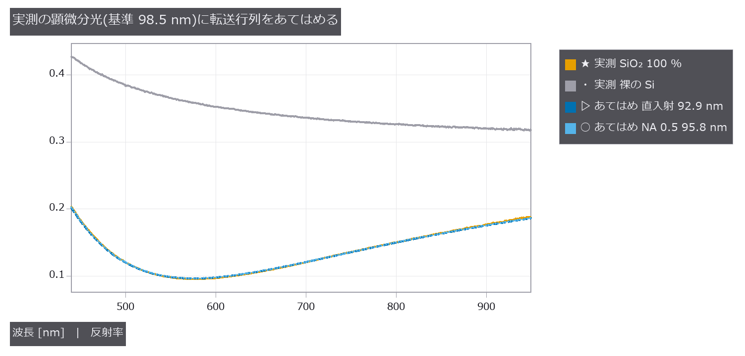
↑ The measurement ―― 実測の反射スペクトルに film_thickness_fit を当てた。直入射のモデルは 92.9 nm、残差が最小の NA 0.5 で 95.8 nm。裸の Si は材料表の Si と中央値 -0.4 % 差。出典: Schwarz ら, Adv. Opt. Mater. (2024) doi:10.1002/adom.202402502、データ Zenodo 10.5281/zenodo.13753754(CC BY 4.0)。改変: 表から 2 本を選び、モデルの曲線を重ねた。 (figure labels are in Japanese; the numbers are the same)

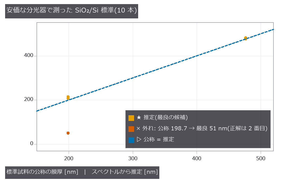
↑ 476.3 nm は最大 1.2 %、198.7 nm は中央値 6.6 % 厚めに読み、1 本は最良の候補が 51 nm に外れた(正しい膜厚は 2 番目の候補)。

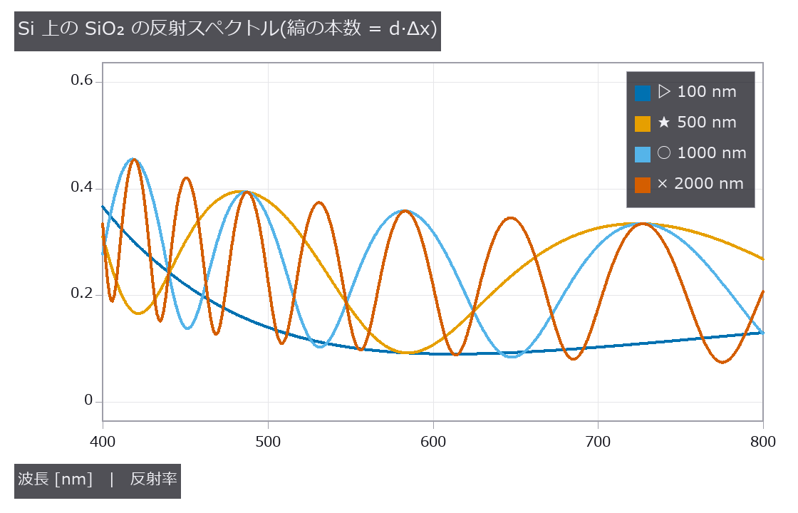
↑ 100 nm は縞が 1 本未満、2 µm は 7 本余り。

↑ 顕微分光の対物は斜めの光も入れる。

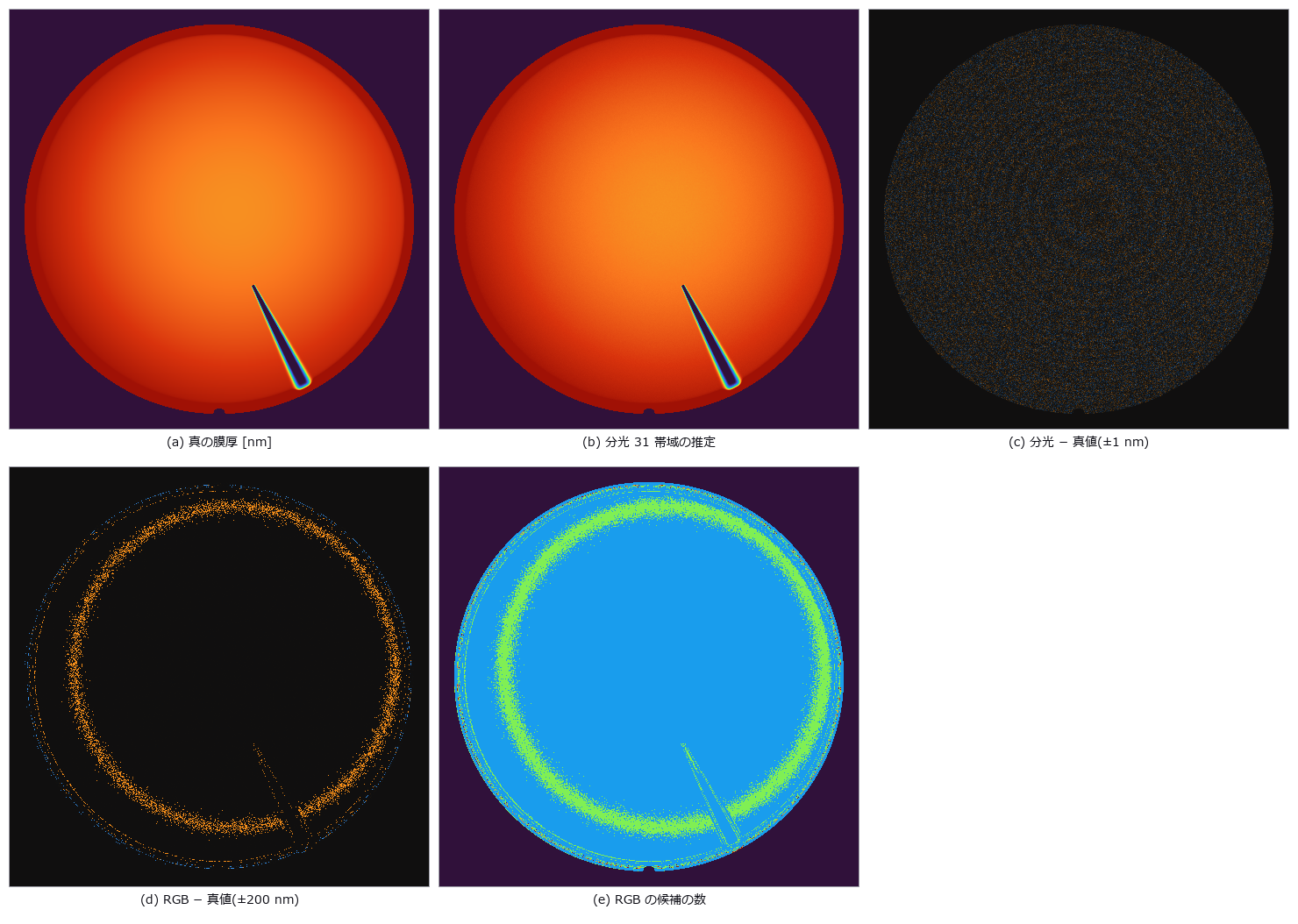
↑ 分光カメラは全画素で真値と RMS 0.17 nm。

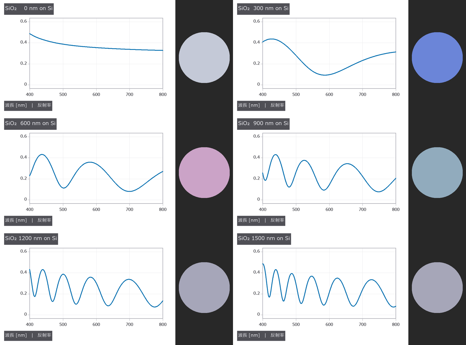
↑ The animation ―― 膜厚を 0 → 1.5 µm に振ると縞が増え、色が周期的に巡りながら淡くなる。

py -3.11 examples/poc_thin_film_reflectometry.py

Source: examples/poc_thin_film_reflectometry.py

This run produced 13 figures in total - see them all

Ops used (notes): annotate_colorbar · blackbody_spectrum · film_color · film_thickness_fft · film_thickness_fit · film_thickness_map · multilayer_reflectance · spectrum · text_box · thinning

No.2026.238 —— Chromatic Confocal Displacement Sensor — A Rainbow Ruler from Glass Dispersion, Reading Height from the Colour that Comes Back

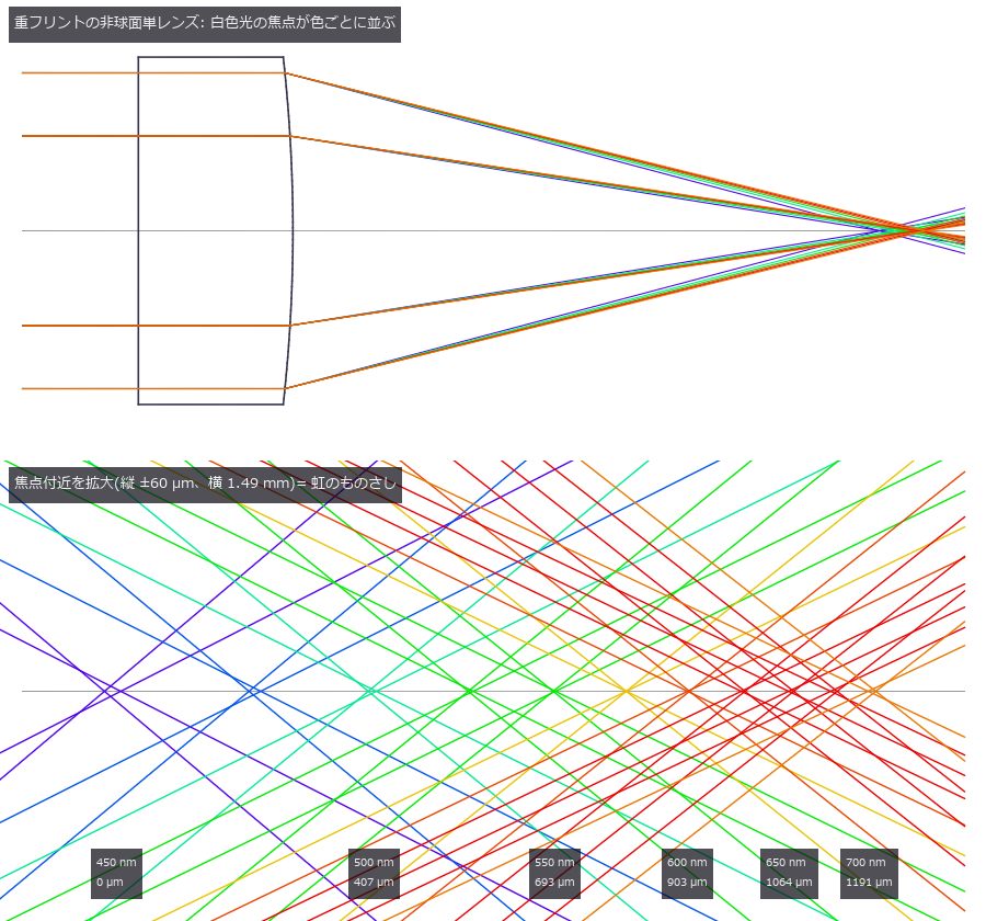
↑ Chromatic Confocal Displacement Sensor — A Rainbow Ruler from Glass Dispersion, Reading Height from the Colour that Comes Back ―― Focusing white light with a lens of strong axial colour puts each wavelength's focus at a different height; only the colour in focus on the surface returns through the pinhole to the spectrometer, so the colour that comes back is the height (Molesini 1984). The sensor is assembled from the objective's prescription (raytrace) and the glass dispersion of the material table (materials), and the measured objects (a borosilicate-crown plate, gold, aluminium, silicon) come from the same table. Six new ops (chromconf, category confocal of opsoptics): the probe calibration (prescription to focus position per wavelength), the confocal axial response (mirror sinc²(u/2), point sinc⁴(u/4), with longitudinal spherical aberration), the return spectrum of a surface and layer stack (Fresnel, tilt, roughness, spectrometer, noise), peak picking, readout of heights and plate thickness, and the closed-form limits. An aspheric dense-flint singlet (V_d 20.9; f 16 mm, NA 0.16) spreads the 450-700 nm foci over 1,191 µm; the paraxial focus matches the thick-lens closed form to 4e-12 µm and the axial response width matches 0.443 λ/(1 − cos α) (∝ λ/NA²). The asphere cancels spherical aberration at 575 nm only: at 450 nm the marginal focus is 40 µm short and the calibrated peak moves by half of that, at 0.74 of the height. A spherical singlet of the same focal length smears the response 29-fold; a hyperchromat (negative fluor crown + positive dense flint) gives 1.63 times the range per focal length. With the design calibration the estimators are biased by 0.060 (Gaussian), 0.108 (parabolic), 0.293 (centroid) and 2.04 µm (peak bin); calibrating by moving a mirror, as a real instrument does, removes the Gaussian bias (0.014 µm) but not the parabolic one (0.090 µm, it oscillates with the bin grid). Under noise the ranking flips: the centroid scales as √N and the Gaussian scatters 4.4 times more. A 500 µm borosilicate-crown plate reads −1.23 µm thin with the paraxial index correction, −0.07 µm with the NA correction and −2.18 µm with the catalogue n_d; four plates (including sapphire and PMMA) are within 0.1 %. Nothing returns from a mirror tilted beyond 8.8-9.5°; gold pulls the reading 0.15 µm far near 509 nm, as the reflectance-slope / response-curvature closed form predicts (dividing by gold's reflectance brings it to 0.005 µm); films under 32 µm merge into one peak (Sparrow: 30.6 µm) and the readout refuses them; a white LED's spectrum biases by 0.93 µm until divided by a white reference (0.014 µm). Real images: from Fig. 6(b) of Qin et al., Sensors 24(20):6649 (2024, CC BY 4.0) the standard groove reads 66.095 µm against the 66.14 µm reference (−0.045 µm) and the paper's own fit of 66.244 µm (−0.149 µm), one figure pixel being 0.33 µm; the raw spectral image of Fig. 3(a) shows the step as 4.0 pixels but carries no µm scale, so this re-reads the paper's result rather than validating the sensor model. Nothing learned, one synthetic mirror calibration, 33 gates (+6 with the real figures).

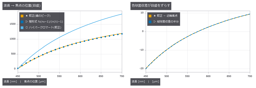
↑ The measurement ―― 左: 単レンズの範囲 1191 µm、ハイパークロマート 1842 µm(焦点距離あたり 1.63 倍)。近軸焦点は閉形式と 4e-12 µm で一致(点)。右: 鏡で較正したピークは近軸焦点から縦球面収差のほぼ半分だけずれる —— 450 nm で -20.0 µm。575 nm では 0(非球面で消した色)。 (figure labels are in Japanese; the numbers are the same)

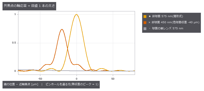
↑ 鏡面の応答は sinc²(u/2)、FWHM = 0.443 λ/(1 − cos α)(∝ λ/NA²)。

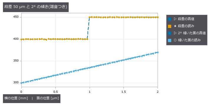
↑ 段差は 49.959 µm と読める(RMS 誤差 0.276 µm)。

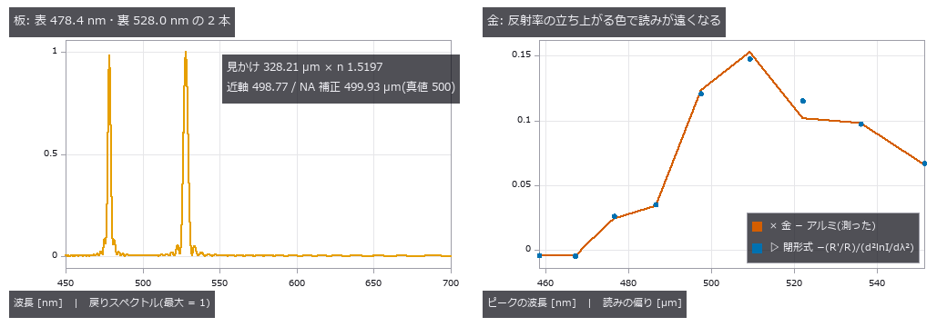
↑ 左: 透明な板は表と裏の 2 ピーク。

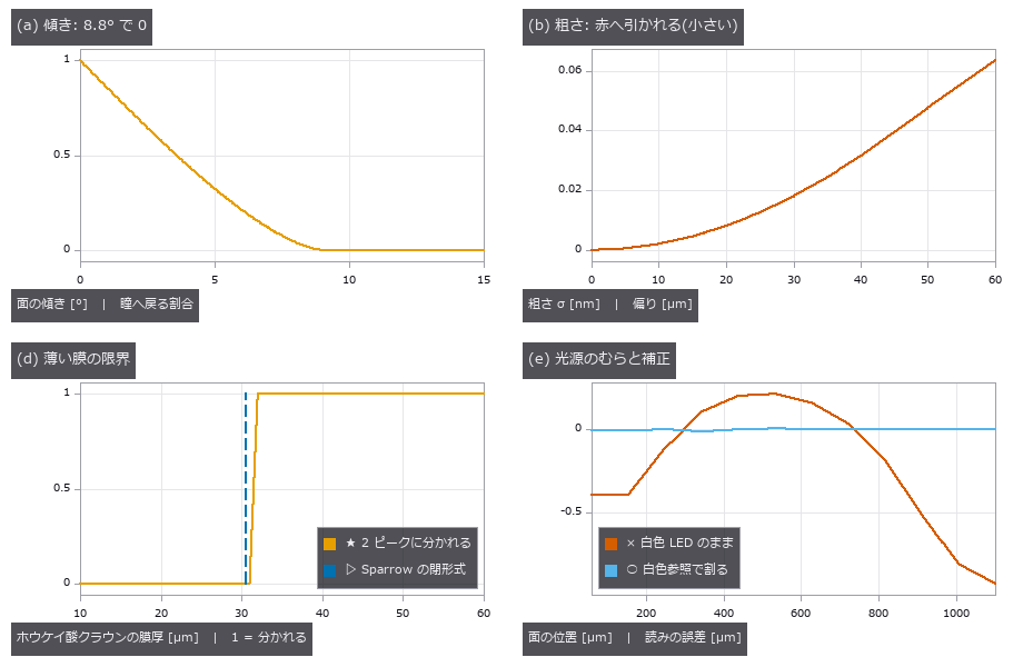
↑ (a) 鏡面の傾きが 8.8°(sin 2θ = 2NA)を超えると何も戻らない(瞳の光線のモンテカルロと一致)。

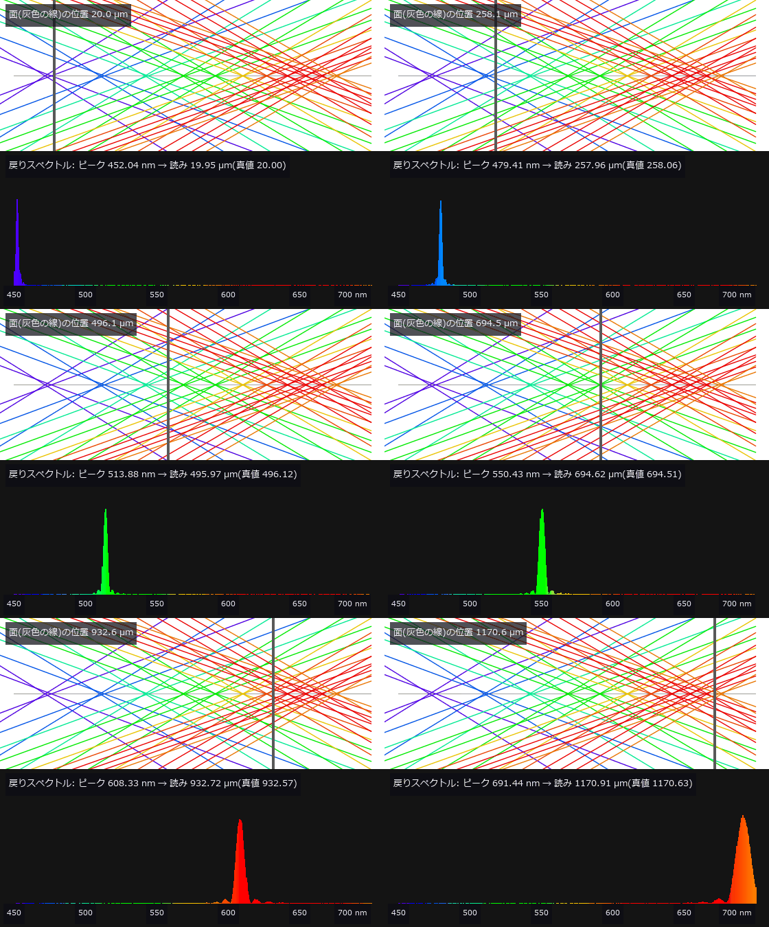
↑ The animation ―― 上: 虹のものさし(焦点付近の光線)と面(灰色の縦線)。下: ピンホールへ戻るスペクトル(棒の色はその波長の色、ピーク 3000 光子 + 読出し雑音)。面を遠ざけると、ピントの合う色が青から赤へ移り、戻る色が変わる。ピーク波長を較正表で引くと高さになる。

py -3.11 examples/poc_chromatic_confocal.py

Source: examples/poc_chromatic_confocal.py

This run produced 8 figures in total - see them all

Ops used (notes): abbe_number · chromatic_confocal_limits · chromatic_confocal_peaks · chromatic_confocal_probe · chromatic_confocal_readout · chromatic_confocal_spectrum · cie_xyz_from_wavelength · confocal_axial_response · gaussian · led_spectrum · lens_system · material_optical_constants · material_reflectance · paraxial_trace · plate_focus_shift · text_box · trace_rays · with_wavelength

No.2026.245 —— A Virtual SEM — Fire Electrons One by One into the Solid, and the Image and the Measured Line Width Change with the Voltage (Scored against Measured Data)

↑ A Virtual SEM — Fire Electrons One by One into the Solid, and the Image and the Measured Line Width Change with the Voltage (Scored against Measured Data) ―― An SEM image is not a photograph of the surface: it is a tally of what comes out of the interaction volume of primary electrons scattering inside the solid. Eight new ops (sem_electron_mc, sem_yield_curve, sem_se_universal_curve, sem_line_profile, sem_cd_measure, sem_image, sem_charging_series, sem_se_escape_fraction) and the material-table op material_electron_properties build a Monte Carlo that tracks electrons one by one (Joy's single scattering, Browning's 1994 Mott fit for elastic scattering, the Joy-Luo stopping power), and every stage is scored against outside measurements. The backscatter coefficient for 7 elements (C to Au) at 5/10/20/30 keV falls inside the measured bands of Joy's database plus or minus 0.04; switching back to screened Rutherford fails for W and Au. The maximum penetration is 0.83 to 1.04 of the Kanaya-Okayama range and the depth grows as E^1.75 (Si) and E^1.52 (Au) against 1.67. The shape of the secondary-electron yield matches the Lin and Joy 2005 universal curve within RMS 0.076 for C to Ag, with Emax within -4 to +7 % of their table (not fitted); W and Au have heavier tails (SE2 dominates, unresolved). The user's guess that W on Si is invisible in SE but stands out in backscatter Z contrast holds only for flush W at 1 kV (SE +5 %, BSE +96 %); at 5 kV SE shows it too (+80 %) because the SE2 made by exiting backscattered electrons carries Z. W buried 150 nm deep shows +3 % at 1 kV even in backscatter and +154 % at 20 kV (information depth). For CD-SEM, a PMMA line (40 nm at the base) with an 88 degree sidewall measures 39.1 nm at 1 kV and 39.9 nm at 20 kV by threshold: low voltage measures high on the sidewall (0.33), high voltage at the foot (0.03); at 80 degrees the difference is small and reversed, so this is no general rule. A vertical sidewall reads wide at every voltage (+0.3 to +1.0 nm). Charging: at 0.5 kV (eta + delta > 1) the insulator charges positive, darkens and stops at the potential that solves eta + delta F(V) = 1 by an independent bisection (to 2e-15 V); at 20 kV it keeps charging negative and brightens (phenomenological). A defect found on the way is kept on record: free paths were drawn in the starting material and walked straight through material boundaries, so a 0.01 nm Si cap changed W's eta from 0.425 to 0.329 (now truncated at the boundary, with a regression gate). No real-image chapter yet: no CC BY CD-SEM images with ground-truth line widths were found.*

↑ The measurement ―― δ(E) を各元素の MC の山(Emax, δmax)で割った形(横軸は対数)。破線は Lin & Joy 2005 の普遍曲線(式 12)。C〜Ag の 5 元素は重なる。W と Au(赤)は E > 3 Emax で裾が厚い —— 重元素は反射電子が多く、表面を抜けるときに作る SE2 が主になるので、SE1 だけを仮定した普遍曲線からずれる(未解決のまま数で固定)。 (figure labels are in Japanese; the numbers are the same)

↑ レンズ内の SE の線プロファイル(基板の水準で割った)。

↑ PMMA の線(高さ 40 nm)を Si の上で。

↑ Si に埋もれた W(幅 100 nm、厚さ 60 nm)の、真上と 400 nm 離れた Si の平均との比 − 1(反射電子 / レンズ内 SE)。

↑ 各パネルは Si の水準で割った信号(0〜3 で共通の濃淡)。

↑ The animation ―― Si の上の PMMA の線を 5 kV で 24 コマ走査し続けた像。PMMA だけが負に帯電して明るくなり、接地した Si は変わらない。

py -3.11 examples/poc_virtual_sem_kv_cd_bse.py

Source: examples/poc_virtual_sem_kv_cd_bse.py

This run produced 9 figures in total - see them all

Ops used (notes): material_electron_properties · sem_cd_measure · sem_charging_series · sem_electron_mc · sem_image · sem_line_profile · sem_se_escape_fraction · sem_se_universal_curve · sem_yield_curve · threshold

No.2026.246 —— A Virtual Transmission Electron Microscope — Thon Rings Move with Focus, Fine Detail Reverses, and Defocus Is Read from Real Micrographs

↑ A Virtual Transmission Electron Microscope — Thon Rings Move with Focus, Fine Detail Reverses, and Defocus Is Read from Real Micrographs ―― A TEM turns the phase of electrons that pass a thin specimen into intensity through the spherical aberration Cs and the defocus Δf. The transfer, CTF = −sin(χ + arcsin w), flips sign with spatial frequency and draws its zeros as concentric Thon rings in the power spectrum. Eleven new ops (temsim, category tem of opsoptics): electron wavelength, Scherzer defocus, 2-D and 1-D CTF, projected potential, amorphous film, weak-phase image, multislice, power spectrum, CTF estimation and correction. Imaging reuses coherent_image with the pupil e^{iχ}, electron scattering factors come from the X-ray factors of pxrd via Mott–Bethe, lomb_scargle seeds the ring period from samples uneven in k², and phase_correlation_fft aligns frames. Wavelengths match the published values to five digits (1.9687 pm at 300 kV; 13.7 % longer without relativity), CTF zeros match the closed form to 1.7e-12 1/Å, the first zero at Scherzer focus is 0.6580 Cs^¼ λ^¾, and a sinusoidal phase grating diffracts as J_n(φ₀)² to 1.6e-13. The mean inner potential of Si is 13.83 V against the neutral-atom 13.71 V (above the measured 12.48 V by the bonding share); Cu's f_e(0) is 10.5 % low, a limit of the X-ray fit. The image best resembles the projected potential at 900 Å, within 7 % of Scherzer's 842 Å, and fine detail reverses at exact focus (correlation −0.30). Four synthetic micrographs give Δf within 13 Å and astigmatism within 50 Å and 5.2°, with jackknife errors that cover the misses; noise only, too low a dose, near-focus and a fit trapped in a wrong valley with only nine tiles are all refused. A 2 % pixel-size error scales Δf by 1.039 (closed form 1.0404). Ten drifting frames lose their rings when summed (fit resolution 15.6 Å) and regain them when aligned (5.3 Å). Phase flipping raises the correlation with the potential from 0.09 to 0.84, Wiener to 0.87, and a 10 % defocus error drops it to 0.10. On three real micrographs (EMPIAR-10028, CC0) the estimate agrees with the authors' CTFFIND3 values to −55, +65 and −0.5 Å (within 0.2 %). Nothing learned, nothing calibrated, 36 gates.

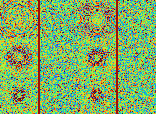
↑ The measurement ―― 焦点外れ Δf を 0.3 → 3 µm と振る(300 kV、Cs 2.7 mm、非晶質炭素 50 Å、40 e/Ų 相当の雑音)。左はパワースペクトル(k ≤ 0.25 Å⁻¹、動径の背景で割った)、右は同じ写真の一部。Thon リングは Δf とともに内側へ詰まり、写真の粒状の模様が細かくなる。 (figure labels are in Japanese; the numbers are the same)

↑ CTF = −sin(χ + arcsin w) に空間・時間の包絡を掛けた曲線(300 kV、Cs 2.7 mm、照明の半角 0.05 mrad、焦点の広がり 60 Å)。

↑ 真値 Δf 25000 Å・非点収差 1500 Å・75° の合成写真。

↑ 10 枚が 1 枚あたり (2.0, 0.6) 画素ずつドリフト。

↑ EMPIAR-10028 part1_001 の 1024 × 1024 画素(1.34 Å/画素)。

py -3.11 examples/poc_tem_ctf_thon_rings.py

Source: examples/poc_tem_ctf_thon_rings.py

This run produced 16 figures in total - see them all

Ops used (notes): tem_amorphous_film · tem_ctf · tem_ctf_correct · tem_ctf_estimate · tem_ctf_profile · tem_image_weak_phase · tem_multislice · tem_power_spectrum · tem_projected_potential · tem_scherzer · tem_wavelength

No.2026.250 —— Spectrometer and Illumination Trains — Where the Bandwidth Comes From, and Whether the Lamp Shows in the Field

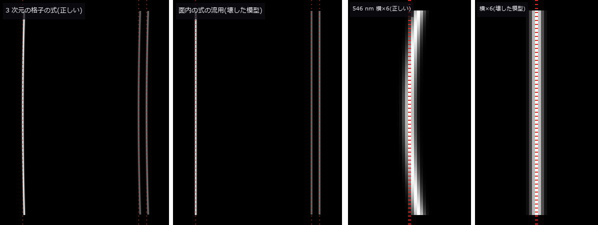
↑ Spectrometer and Illumination Trains — Where the Bandwidth Comes From, and Whether the Lamp Shows in the Field ―― The hyperspectral PoC used a 10 nm band and the chromatic confocal PoC a spectrometer line width as given numbers. This exhibit builds those numbers from the entrance slit, the grating grooves, the mirror focal lengths and the detector pixels with the grating equation, and the unevenness of microscope and coaxial lighting from which plane of the source is imaged where. Eight new ops: in gratingspec (new category spectrometer of opsoptics) the grating equation with dispersion, resolving power mN and overlapping orders; the first-order Czerny-Turner design with Shafer's coma condition; the bandpass as the FWHM of slit image, pixel and diffraction convolved, with the etendue; smile and keystone from the 3-D grating equation that keeps the direction cosine along the grooves; and the detector reading of an input spectrum with second- and third-order overlap. In illumdesign: the Koehler or critical illumination train, the specimen irradiance by paraxial backward tracing to the source, and the coaxial half mirror with its round-trip R·T and the image of a mirror-like or matte part. Against two published spectrometers (CC BY 4.0 papers) the Shafer angle comes out 14.9679° (published 14.968°), the camera focal length 68.88 mm (r = 136 mm), the slit-image widths 39.2 / 43.7 / 52.6 µm (40 / 43 / 50) and the resolution 0.397 nm (0.385 to 0.391); only the 0.4 nm centre resolution of Feng 2021 disagrees, the slit image alone giving 0.49 nm from the paper's own values, and the gap is left open. Narrow slits stop at the diffraction floor 0.886 λ/(mN) (within 5e-4 for a rectangular pupil), wide slits keep light times resolution constant; the mercury pair at 576.96 / 579.07 nm splits with a 50 µm slit and merges into one false peak at 150 µm. A 4 mm slit image bows 41.9 µm (3 pixels) towards longer wavelengths, within 0.2 % of the closed form, and the Littrow curvature radius matches f/(2 tan β); a broken model that reuses the in-plane equation shows no smile and fails the gate. The 253.65 and 365.02 nm mercury lines appear in second order as false lines at 507.30 and 730.04 nm and vanish behind a 400 nm long-pass filter. For an InGaAs spectrometer at 900 to 1700 nm the hyperspectral 10 nm corresponds to a 75 µm slit (trapezoidal, not Gaussian). Widening the visible spectrometer slit of the chromatic confocal sensor merges the two surfaces of thin glass plates until the readout refuses them. Critical illumination copies a coiled filament into the field (CV 0.53), Koehler illumination removes it (CV 2e-16), and moving the aperture stop 4 mm off the condenser focal plane lets the stripes leak back. The coaxial round trip is R·T = 1/4 at 50/50, matching the optscene coaxial light. Nothing learned, nothing calibrated, 40 gates.

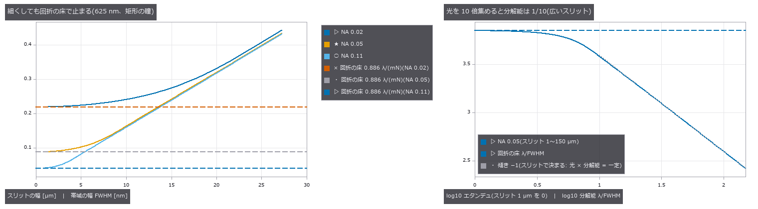
↑ The measurement ―― スリットの幅で帯域の幅とエタンデュがどう動くか(1200 本/mm、M 型 2025 の設計、625 nm)。左: 細いスリットは回折の床 0.886 λ / (mN) で止まり、NA を上げて照らす溝を増やすと床が下がる。右: 広いスリットでは光の量と分解能の積が一定(傾き −1)、細くしていくと床に当たって光だけを失う。 (figure labels are in Japanese; the numbers are the same)

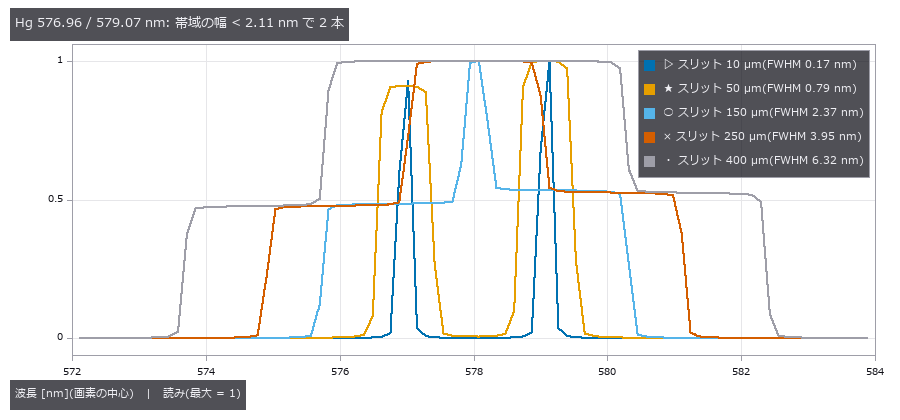
↑ Hg の黄色の 2 本を、スリットの幅を変えて読む。

↑ 1 次の 500〜750 nm の検出器に、紫外の Hg 線の 2 次の像が偽の線として乗る(効率 0.3 の模型)。

↑ 可視の分光器(600 本/mm)のスリットを広げると、薄い板の表裏の 2 ピークが 1 つに潰れ、readout は厚さを当て推量せず拒否する。

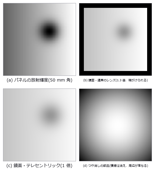
↑ 同軸落射(視野 44 mm 角): 鏡面の部品はパネルそのものを写す(R·T = 1/4)。

py -3.11 examples/poc_spectrometer_illumination.py

Source: examples/poc_spectrometer_illumination.py

This run produced 10 figures in total - see them all

Ops used (notes): chromatic_confocal_peaks · chromatic_confocal_probe · chromatic_confocal_readout · chromatic_confocal_spectrum · coaxial_illumination · czerny_turner_design · grating_dispersion · illumination_field · illumination_train · spectrometer_bandpass · spectrometer_slit_image · spectrometer_spectrum · text_box · wave_grating_orders

No.2026.251 —— Grating Interferometry — Fibre Orientation, Micro-Cracks and Pores That Absorption Cannot See, Read From the Fringe Amplitude (Dark Field)

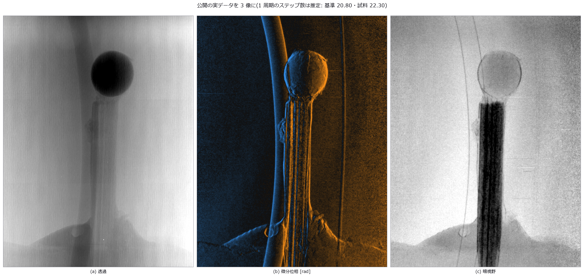
↑ Grating Interferometry — Fibre Orientation, Micro-Cracks and Pores That Absorption Cannot See, Read From the Fringe Amplitude (Dark Field) ―― A grating interferometer's dark field (the loss of fringe amplitude) shows what absorption hides: fibre orientation, a 2 µm crack and a cluster of pores. Eight new ops (gratinginterf, category grating_interf of opsoptics): closed-form design (fractional Talbot distances for π, π/2 and absorption gratings, the cone-beam distance d' = Ld/(L − d), analyser and Lau source-grating periods), the Talbot carpet I(x, z) as a sum over diffraction orders, the visibility loss from source size, Gaussian focal spots and source gratings, a phase-stepping forward model, estimation of the steps per period from the sine-fit residual, retrieval of transmission, differential phase and dark field from sample and reference stacks, dark field to scattering width, and integration of the differential phase into phase and thickness (refusing wrapped input). The four visibility maxima of the carpet sit on the fractional Talbot distances (m − 1/2)p²/(4λ) to within the 0.89 mm grid, at height 1.2732 (4/π for a square wave), and agree with an FFT propagation of the sampled field to 8e-4. A 2 mm focal spot washes the fringes out to x0.001; a source grating at the Lau period (41 slits) restores 2/π = 0.637, and detuning it by 1/41 kills them again (matching an incoherent point sum to 6e-5). In a short-fibre composite plate the 2 µm crack reaches CNR 13.5 in the dark field against 1.34 in absorption, the cos 2ω of four grating directions recovers fibre orientation to a median 2.7° (90th percentile 6.6°), and the weld line behind the hole reads 89.8° for 90°. Probe: with only 0° and 90° the diagonal fibres are off by 30.3°. Integrating the differential phase recovers a rod's thickness to 1.0 %, and the op refuses once the true |φ| exceeds π. Honest limit: a slab whose sharp edge pushes a single pixel past π wraps invisibly and the op silently returns -857 µm for 2000 µm. Assuming P = N for a scan of 20.85 steps per period leaves 0.063 rad of phase error, the estimated P 0.022 rad; dividing the residual by the fitted mean biases the minimum by +0.03 steps (the op divides by the raw mean). Real data (CC BY 4.0, Zenodo 16944391): 20.80 and 22.30 steps per period for the 22-frame reference and 24-frame object scans (residual 0.0073 to 0.0044); the strongly absorbing sphere scatters little (-ln D 0.17) while the fibre bundle scatters strongly (0.55), and the differential phase changes sign across the sphere. Nothing learned, nothing calibrated, 22 gates (with the real-data chapter run; 19 when the data is absent, as in CI).

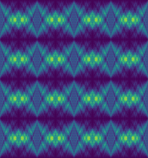
↑ The measurement ―― 位相 π の格子(28 keV、p1 = 4.36 µm)の後ろの強度 I(x, z)。横 = 第 1 格子からの距離 0〜z_T/2(429 mm)、縦 = 2 周期。周期 p1/2 の縞が結ぶ距離が分数タルボ距離 (m − 1/2)p1²/(4λ) = 54, 161, 268, 376 mm。z = 0 は純粋な位相格子なので強度は一様(縞が無い)。 (figure labels are in Japanese; the numbers are the same)

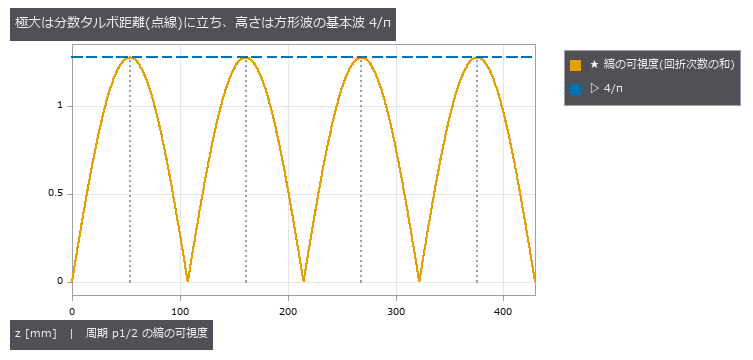
↑ 点線 = 閉形式の距離。

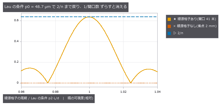
↑ 開口 1/2 の線源格子。

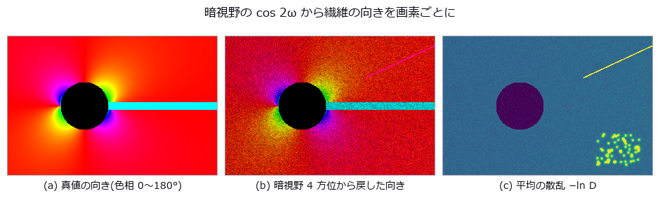
↑ 中央: 色相 = 向き、明るさ = 異方性の強さ。

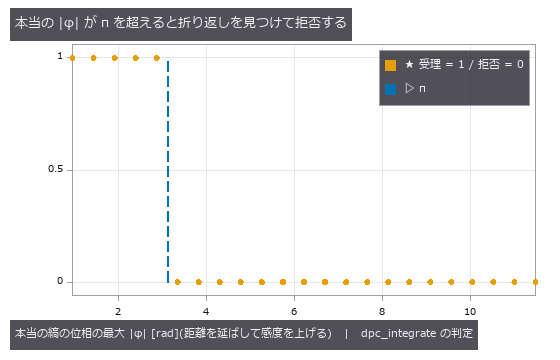
↑ 正直な限界: 鋭い縁の 1 画素だけが π を超える板は、折り返した値が背景と π 以内に収まるので見えずに通る(中央の厚さ -857 µm、真値 2000 µm)。

↑ The animation ―― 格子の向きを 0〜180° に回したときの暗視野(4 方位から戻した a、b、θ で描く)。繊維が格子の感度の向きに直交すると暗くなり、明暗の帯が向きの場に沿って流れる。

py -3.11 examples/poc_grating_interferometry.py

Source: examples/poc_grating_interferometry.py

This run produced 12 figures in total - see them all

Ops used (notes): angular_spectrum_propagate · dpc_integrate · grating_step_period_estimate · grating_stepping_simulate · grating_three_image_retrieve · talbot_carpet · talbot_grating_design · talbot_source_visibility

No.2026.255 —— Bone and Glass in Meat, Separated by Material with Two X-ray Energies (Dual-Energy and Photon-Counting X-ray)

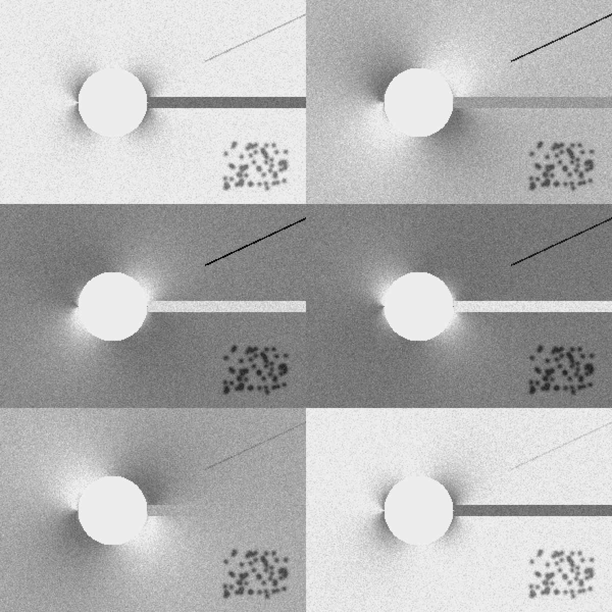
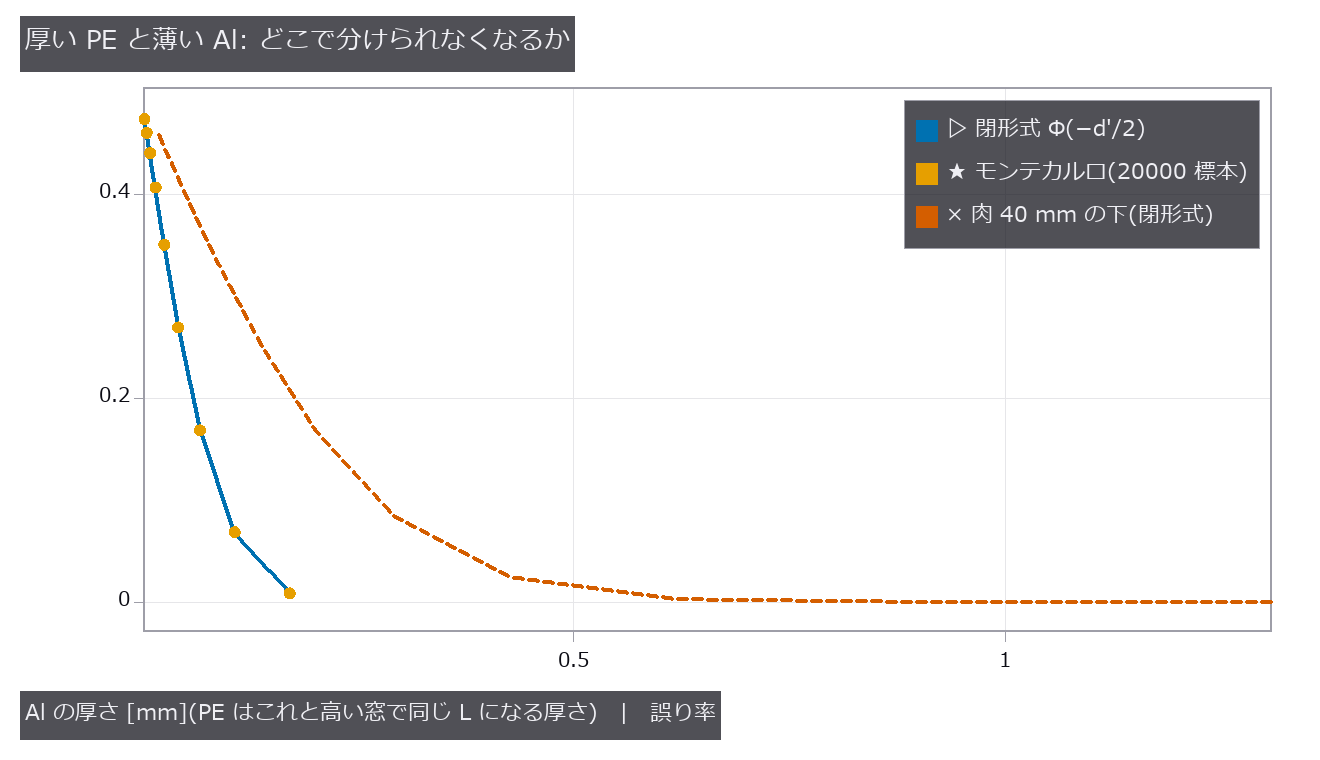
↑ Bone and Glass in Meat, Separated by Material with Two X-ray Energies (Dual-Energy and Photon-Counting X-ray) ―― A single X-ray transmission image of food measures one number per pixel, L = -ln(I/I0), so a thick piece of meat and a thin hard foreign body cannot be told apart. A detector that counts photons in two energy windows can: the shape of mu(E) differs by material, so thickness and material separate in every pixel (the Alvarez and Macovski 1976 basis decomposition). Fourteen new ops (spectral_xray in opstomography): the X-ray columns of the material table (material_xray_attenuation and three more, a subset of NIST SRD 126 plus a mixture rule) and ten dualxray ops (tube spectrum, beam quality, detector channels, projection, basis decomposition, CRLB, R value, effective Z, discrimination error rate). mu/rho matches the NIST published values (Cu at 8 keV 52.55; across the K edge 38.4 to 278.4), and the tube model's half-value layers agree with the eight IEC 61267 qualities to within 5.8 % (the model was shaped on a public spectrum calculator (MIT); the IEC values were not used to fit it). On a meat tray 25 to 60 mm thick the bone-and-glass step is 0.9 times the meat unevenness, one threshold flags 86 % of the meat, and even the high band shows two false lumps at the edge of a meat overlap, whereas the Al image from a lean-meat plus Al decomposition has 0 false lumps. A confounded pair of thick PE and thin Al gives d' = 0 in one window; the two-window error rate Phi(-d'/2) agrees with Monte Carlo to 0.004, and the Al thickness below which they cannot be separated (5 % error) is 0.125 mm in closed form and 0.126 mm measured, 0.364 mm under 40 mm of meat. The decomposition noise reaches 0.995 and 0.997 times the Cramer-Rao bound. How it breaks: decomposing without knowing 25 % charge sharing turns meat into Al, and a monochromatic approximation biases Al by -1.5 mm under 6 cm of meat; the apparent Z of a buried foreign body also moves with density (PVC at 13.9 reads as 18.7). Learning 0, calibration 0, 21 gates.

↑ The measurement ―― W 陽極の管(Kramers の厚い陽極 + 自己吸収 + K 線 59 / 67 keV)を Al 2.5 mm で濾した光子スペクトル(半価層 2.74 mm Al、平均 42.6 keV)。CdTe 2 mm の吸収効率をかけ、堆積エネルギーで 2 つの窓に分ける。 (figure labels are in Japanese; the numbers are the same)

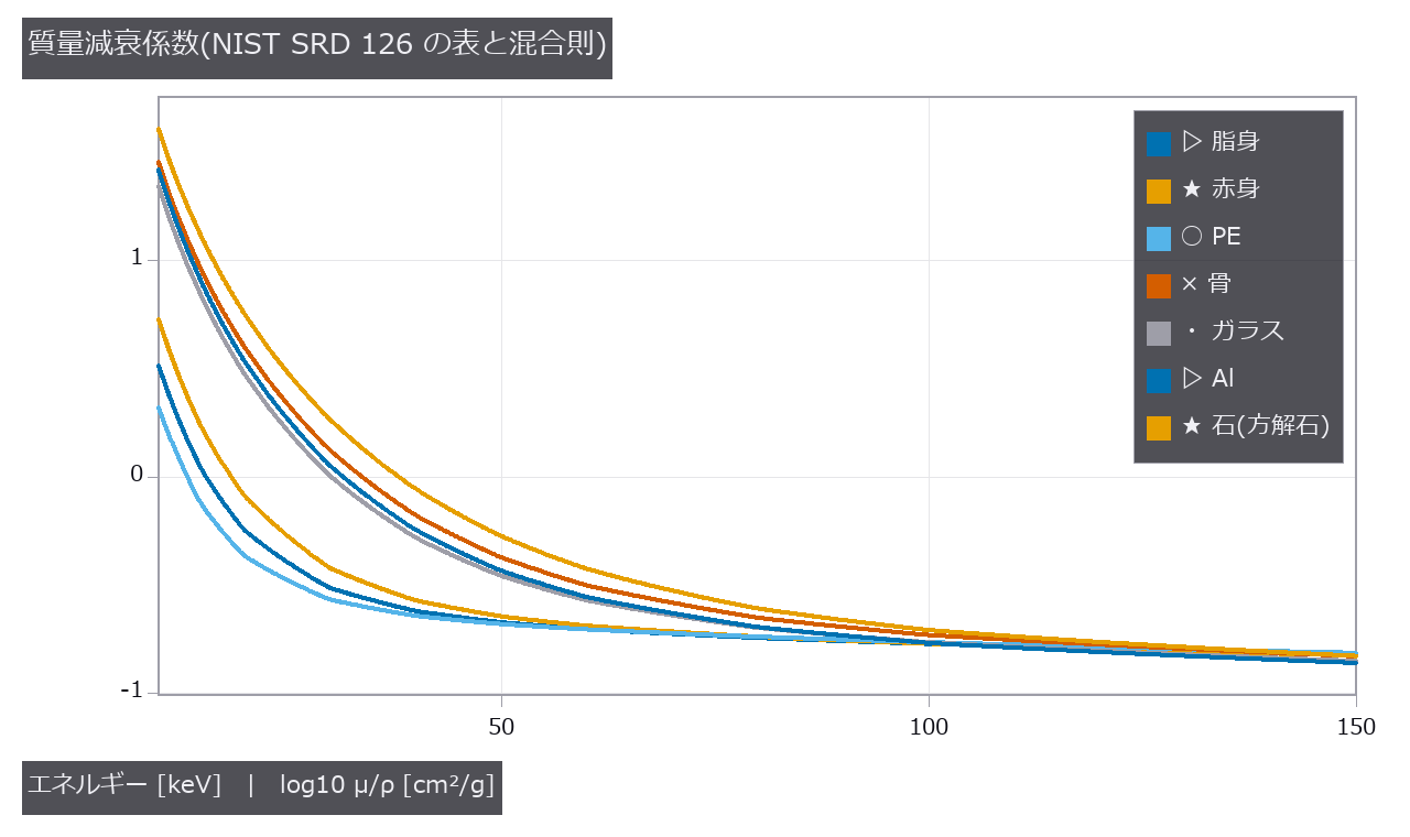
↑ 低いエネルギーでは光電効果(≈ Z³/E³)で Z の大きい材料ほど急に増え、高いエネルギーではコンプトン散乱で電子密度に揃う。

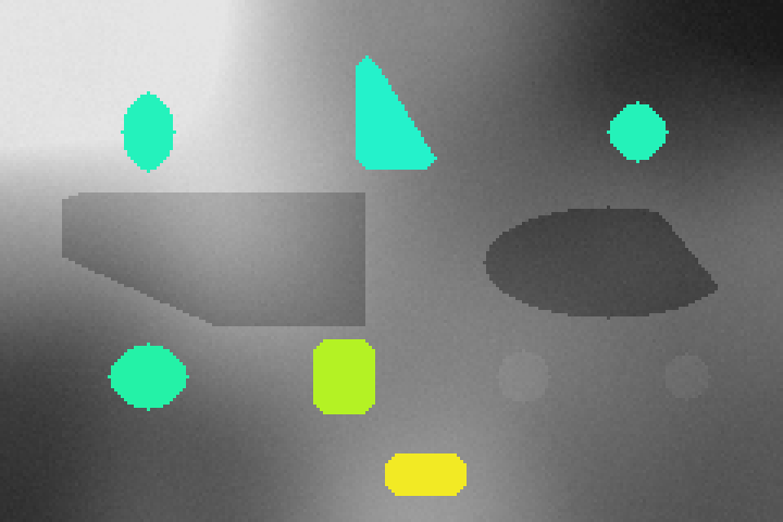
↑ 1 枚の透過像(灰色)の上に、Al の像で浮いた画素だけ、基底の向きから読んだ見かけの Z を色で重ねた(緑 ≈ 12〜14、黄〜橙 ≈ 15〜20、赤 ≈ 25 以上)。

↑ 高い窓だけでは同じ L(1 枚の像の d′ = 0)。

↑ 肉 4 cm の下の Al の厚さの雑音(下限)。

py -3.11 examples/poc_dual_energy_xray.py

Source: examples/poc_dual_energy_xray.py

This run produced 12 figures in total - see them all

Ops used (notes): basis_decomposition_crlb · basis_material_decompose · dual_energy_separability · dual_kvp_channels · ellipse · material_effective_z · material_from_sellmeier · material_xray_attenuation · material_xray_constants · photon_counting_channels · reflect · xray_beam_quality · xray_channel_projection · xray_tube_spectrum

No.2026.271 —— Budgeting Lens Manufacturing Tolerances through MTF, Yield, and Compensator Travel

↑ Budgeting Lens Manufacturing Tolerances through MTF, Yield, and Compensator Travel ―― A public triplet prescription receives explicit rows for curvature, thickness, refractive index, Abbe number, decentre, tilt, astigmatic surface irregularity, wedge, and group decentre. Eight new operations combine distributions, central-difference sensitivity, Monte Carlo, a Wilson 95% yield interval, multiple compensators, and assembly travel. The weak-wedge image shift agrees with f(n-1)alpha to 6e-8; the real-ray OPD RMS of one fringe of astigmatic irregularity agrees with the closed form to 1.3%. In the 16-trial CI run yield is 0.688 and becomes 1.000 with inner-gap and image-plane compensation. Uniform, normal, and truncated-normal distributions at the same plus/minus tolerance yield 0.750 / 1.000 / 1.000; tightening the leading row while loosening low-sensitivity rows gives 0.833. Learning 0, calibration 0.

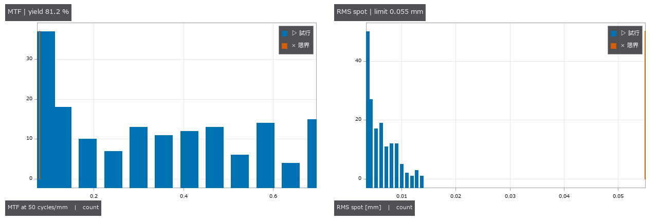
↑ The measurement ―― 同じ試行から得た MTF と RMS spot。赤線は合否限界。 (figure labels are in Japanese; the numbers are the same)

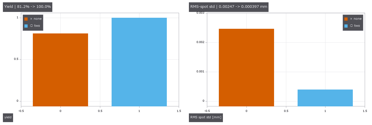
↑ 像面だけの場合と内部間隔を加えた場合を比較。

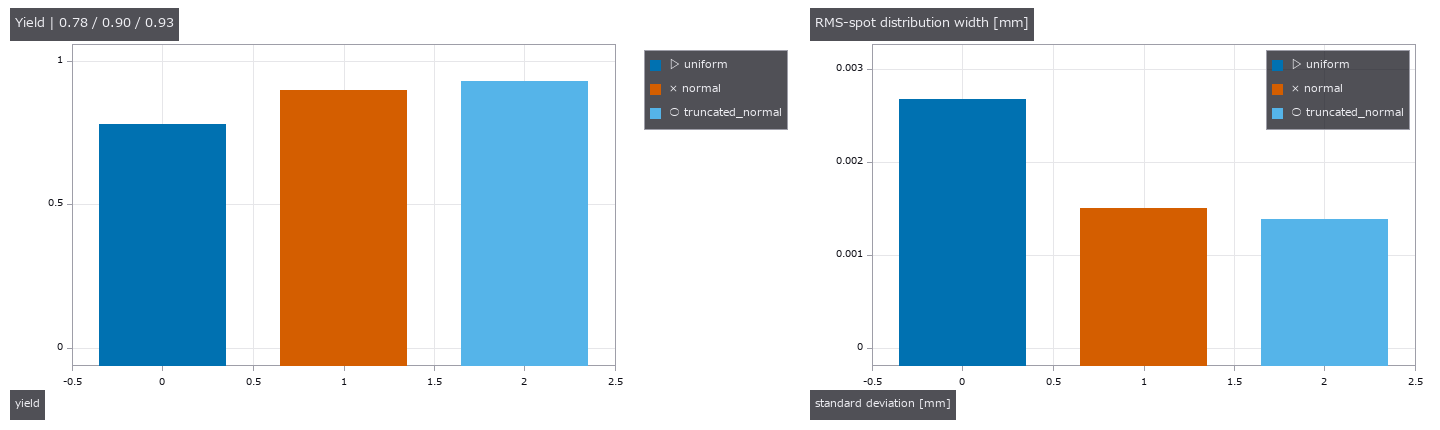
↑ 一様・正規・±公差で切った正規分布の歩留まり。

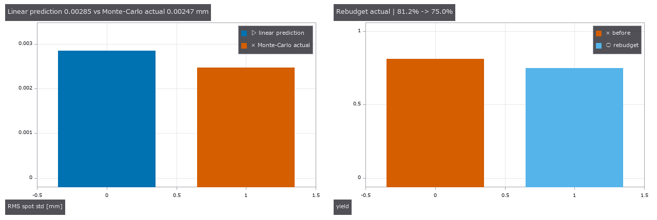
↑ 線形予測と Monte-Carlo 実測を明示。

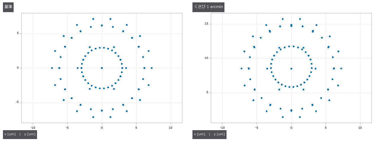
↑ 同じ処方の基準像と、1 arcmin のくさびを入れた像。

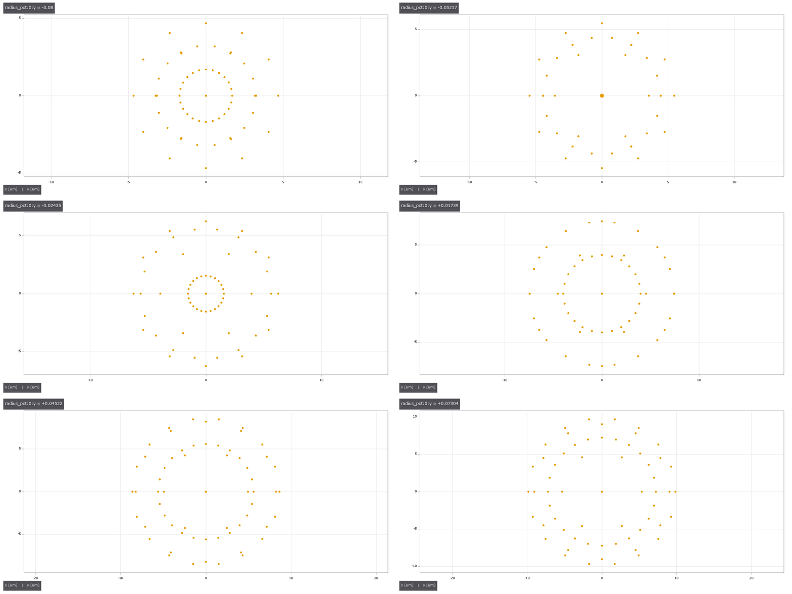
↑ The animation ―― 感度首行を -tol から +tol へ掃引した点像。

py -3.11 examples/poc_lens_tolerancing.py

Source: examples/poc_lens_tolerancing.py

This run produced 7 figures in total - see them all

Ops used (notes): chief_ray · lens_system · opd_samples · ray_bundle · tolerance_compensators · tolerance_criteria · tolerance_monte_carlo · tolerance_report · tolerance_sensitivity · tolerance_table · tolerance_table_from_zmx · tolerance_table_zmx

No.2026.272 —— A Prescription-Based Plenoptic Camera

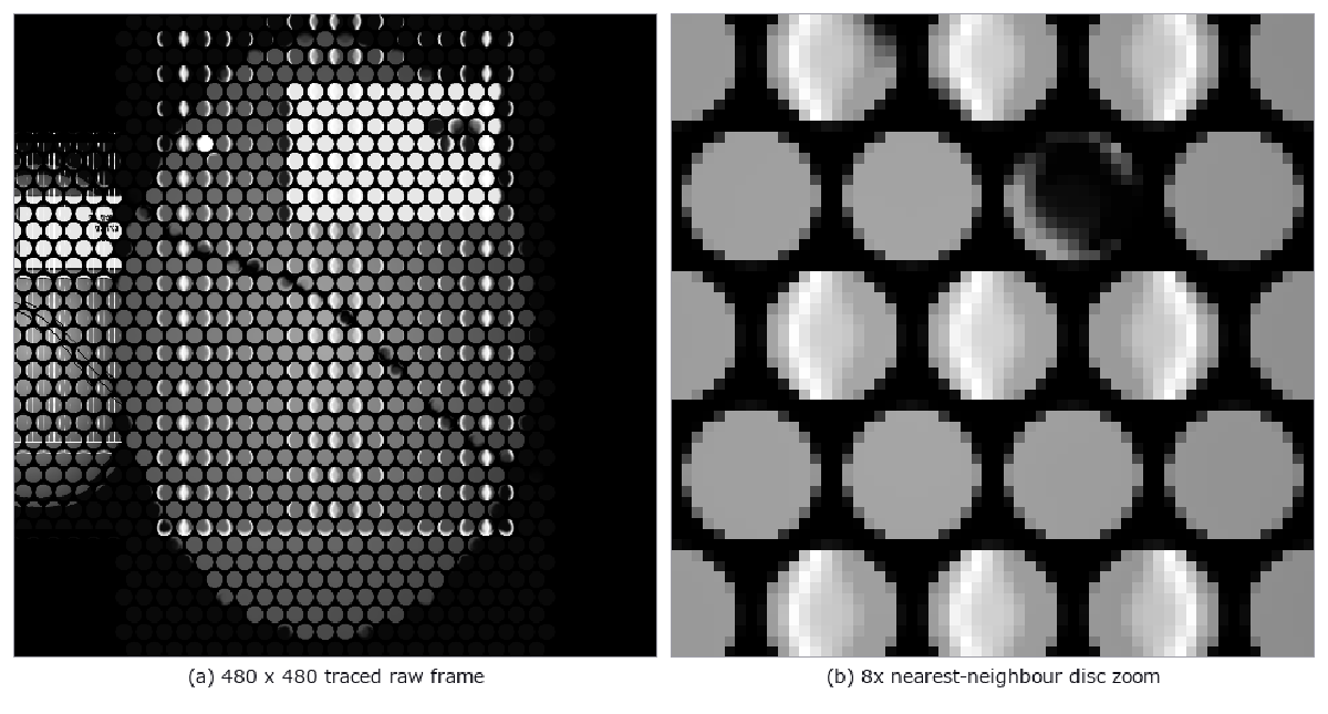
↑ A Prescription-Based Plenoptic Camera ―― A synthetic prescription-based camera traces a main lens, periodic spherical MLA and sensor backwards. Its raw frame shows the three physical signatures: a lattice of microimage discs, dark inter-disc corners, and shifted scene fragments inside each disc; decoding adds slanted disparity lines in the EPI. The white-frame gates measure 21.33% dark corners (closed form 21.46%), a 9.92e-6 rim/core intensity ratio, a 0.06667 cycle/pixel lattice peak, and 0.6 px/view EPI motion. Removing the aperture gives 0% dark corners and fails the gate; boundary rays and excessive calibration residuals also fail closed.

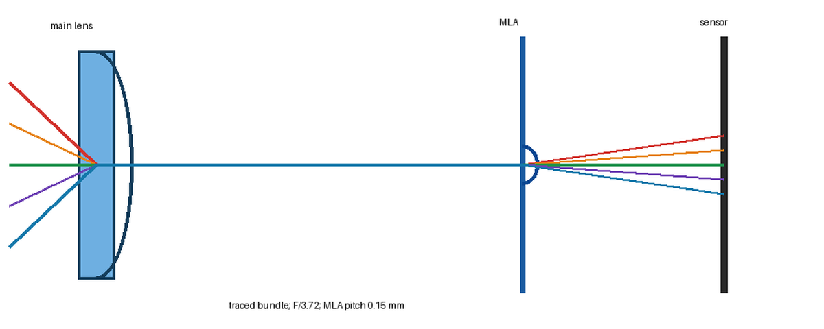
↑ The measurement ―― 480 x 480 sensor, 32 x 32 MLA, 15 pixels per microlens; five prescription-traced rays. (figure labels are in Japanese; the numbers are the same)

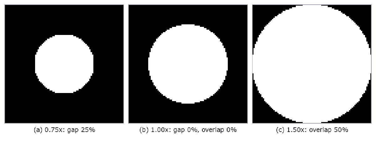
↑ F-number ratios 0.75, 1.00 and 1.50; matched diameter/pitch = 1.000.

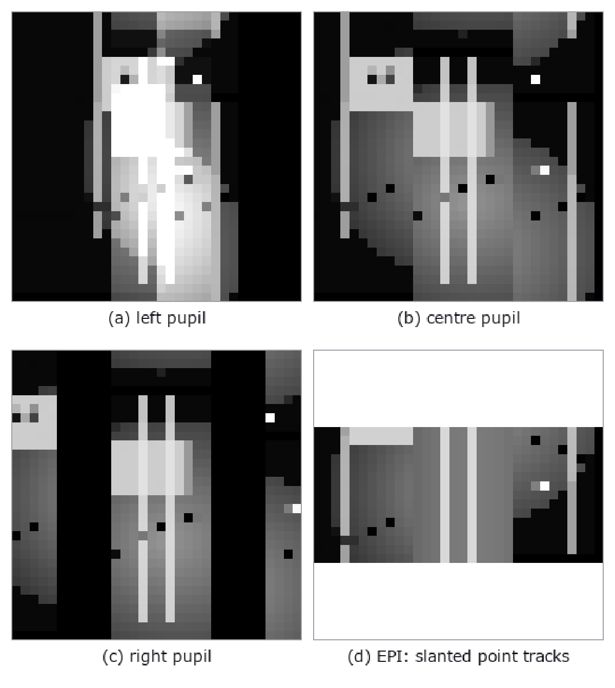
↑ 15 x 15 decoded views; EPI disparity is 0.6 px per view step.

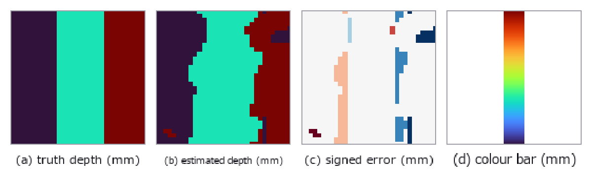
↑ Truth and estimate at 600, 1000 and 1800 mm; signed error and colour bar.

↑ Same MLA: plenoptic 1.0 images the pupil; focused 2.0 images scene fragments.

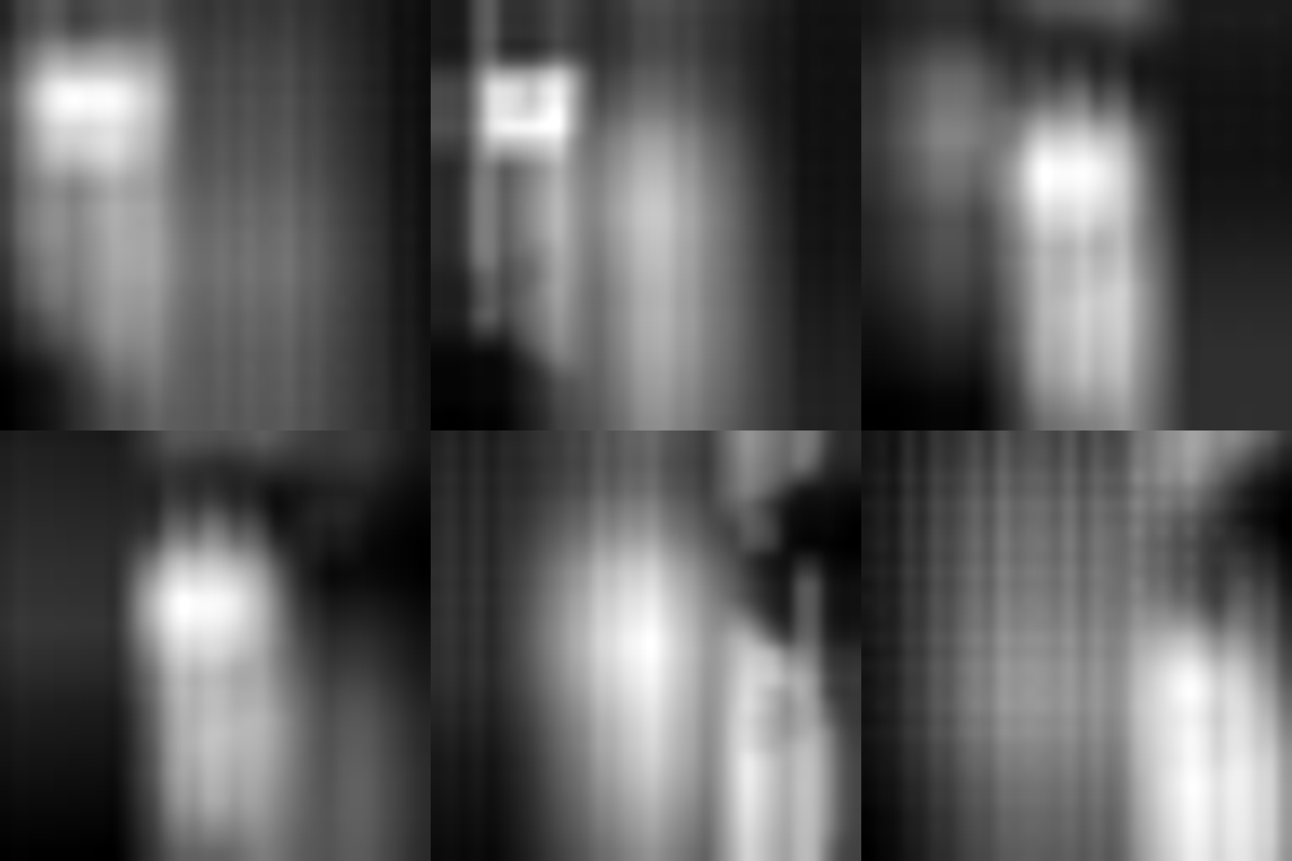
↑ The animation ―― 24-frame 480-pixel refocus sweep; all frames pass the content gates.

py -3.11 examples/poc_plenoptic_camera.py

Source: examples/poc_plenoptic_camera.py

This run produced 9 figures in total - see them all

Ops used (notes): lens_scene · lens_system · lf_depth_from_focus · lf_refocus · mla_surface · paraxial_trace · plenoptic_capture · plenoptic_mla_calibrate · plenoptic_refocus_depth · plenoptic_system

No.2026.273 —— Measuring the Same Particles in Scanning and Transmission Images — Which Is Right, 52 nm or 48 nm?

↑ Measuring the Same Particles in Scanning and Transmission Images — Which Is Right, 52 nm or 48 nm? ―― One ledger of fourteen spherical and faceted particles drives both images. Area-equivalent diameter, maximum slope, watershed splitting of touching pairs, stereo height and limited-angle reconstruction are scored against the shared truth. For a 52 nm particle the scanning-image threshold is +4.16 nm, the transmission image is -0.18 nm at focus and +9.82 nm at 12000 nm defocus. The scanning bias follows the closed-form Gaussian rim width 2 sqrt(2 ln 2) sigma, while the dark transmission fringe follows sqrt(lambda defocus) within ten per cent. Material contrast is checked against published backscatter coefficients; 3-D measurements are checked against parallel-projection geometry and a full-angle reconstruction. No new operators, no learning and no calibration.

↑ The measurement ―― Truth height only: turbo-like pseudo-colour with a nanometre colour bar in the margin. (figure labels are in Japanese; the numbers are the same)

↑ Bright-field in-focus and under-focus output | derived diameters | absolute residual.

↑ この回の図

↑ この回の図

↑ この回の図

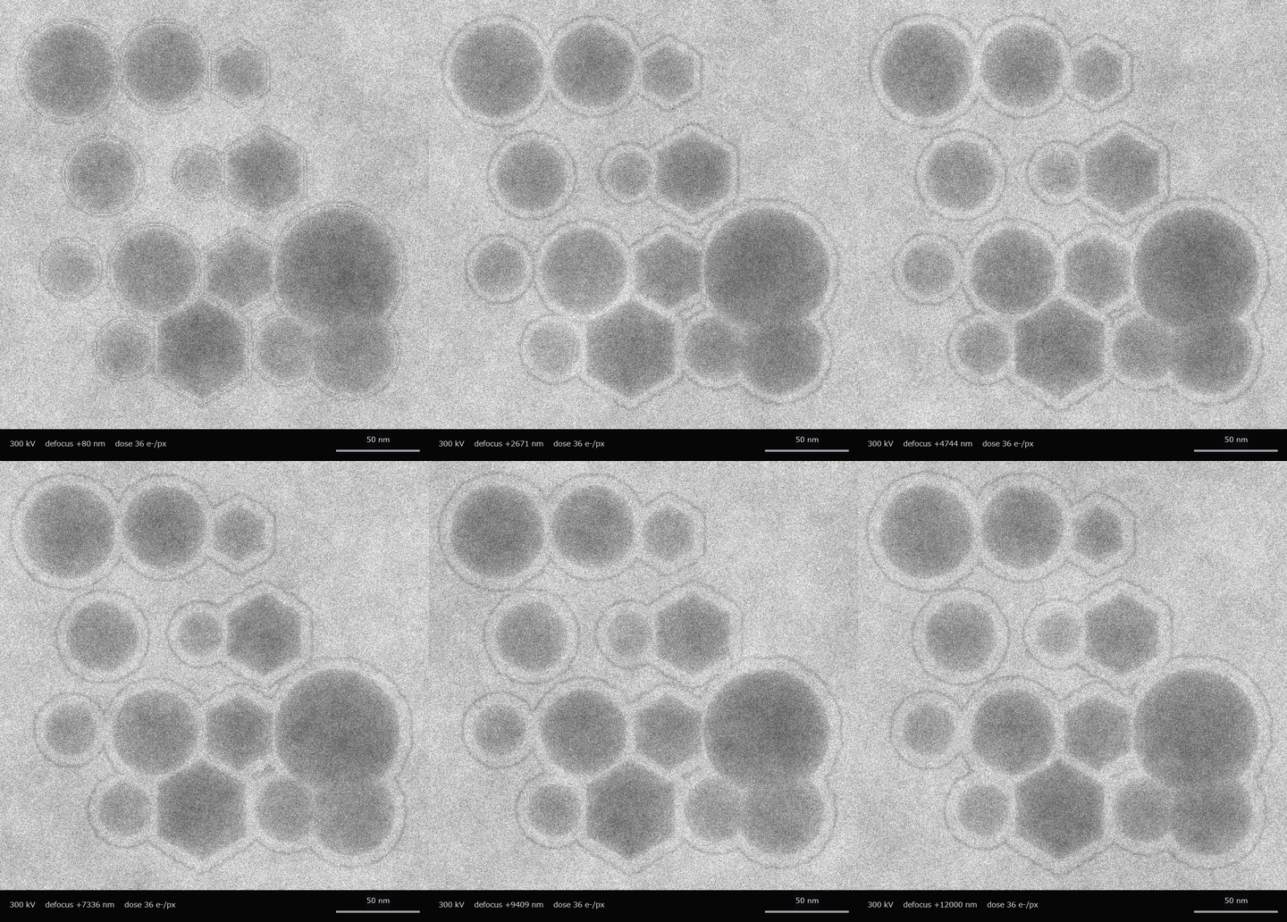
↑ The animation ―― 24 greyscale bright-field frames with data bar; first and last defocus differ

py -3.11 examples/poc_sem_tem_same_particle.py

Source: examples/poc_sem_tem_same_particle.py

This run produced 8 figures in total - see them all

Ops used (notes): color_bar · filtered_backprojection · radon_transform · reflect · scale_bar · sem_electron_mc · sem_image · sem_render · tem_image_weak_phase · tem_multislice · tem_projected_potential · tem_wavelength · text_box · watersheds_marker

No.2026.274 —— Indirect and Direct Time of Flight on One 3-D Scene — Multipath, Mixed Pixels, Pile-up and Volume Error

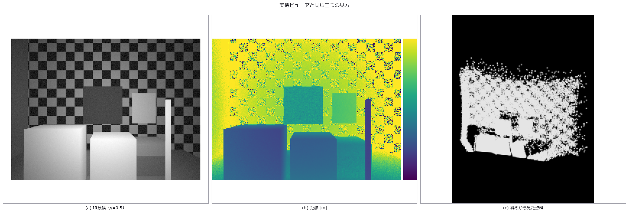
↑ Indirect and Direct Time of Flight on One 3-D Scene — Multipath, Mixed Pixels, Pile-up and Volume Error ―― The same 320 by 240 scene is shown as IR amplitude, colour-coded distance over 1.5–6.0 m, and a point cloud. The amplitude-distribution W1 distance between synthesis and measurement is 0.145 (gate 0.594). The remaining figures add physical effects one at a time; compare amplitude with range noise (log slope -0.878 in measurements and -1.027 in synthesis); reproduce wall-junction bowing (-551 mm measured and +75 mm synthetic, with matching signs after aligning profile direction); separate transparent-pane returns 1.35 m apart; expose mixed pixels around a thin pole; show direct time-of-flight histograms and decoded depth; and tabulate three box-volume errors (+0.16, +0.47 and +0.29 percent). The final animation is a 48-frame, 576 by 432, 8 fps light front moving from 1.4 to 6.2 m. Real frames are not redistributed: only curves and aggregate measurements are shown. No new ops, no learning, no calibration, 13 gates.

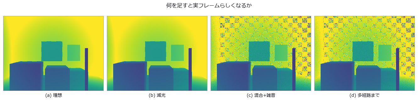
↑ The measurement ―― 全パネル同じ距離範囲。暗部の荒れと隅の湾曲が順に現れる。 (figure labels are in Japanese; the numbers are the same)

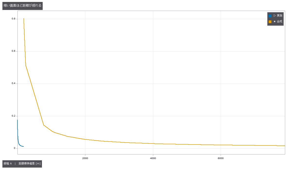
↑ 対数傾きは実測 -0.878、合成 -1.027。

↑ 実測は曲線だけを掲載し、フレームを再配布しない。

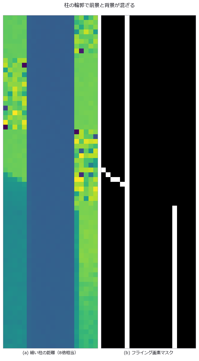
↑ 手描きマスクではなく3×3サブ光線のフェーザ和。

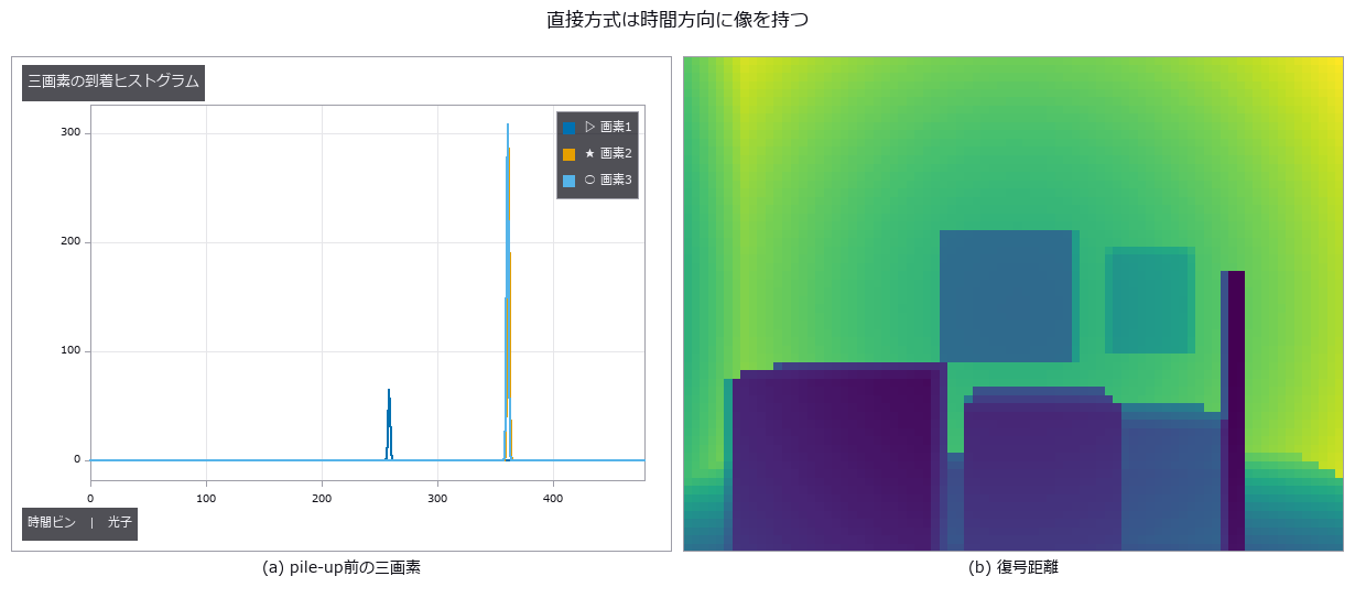
↑ 強い画素では最初の光子が早い側へ偏る。

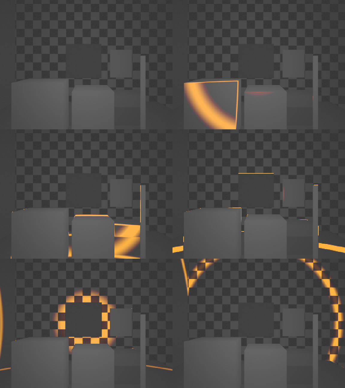
↑ The animation ―― 48枚、576×432。各時刻を99パーセンタイル・γ=0.5で階調化。

py -3.11 examples/poc_tof_camera.py

Source: examples/poc_tof_camera.py

This run produced 9 figures in total - see them all

Ops used (notes): bilateral_filter_depth · depth_to_points · dtof_cube_depth · dtof_cube_simulate · points_render · threshold

No.2026.275 —— Measurable Omnidirectional Inspection, Stereo Display and Moving Viewports

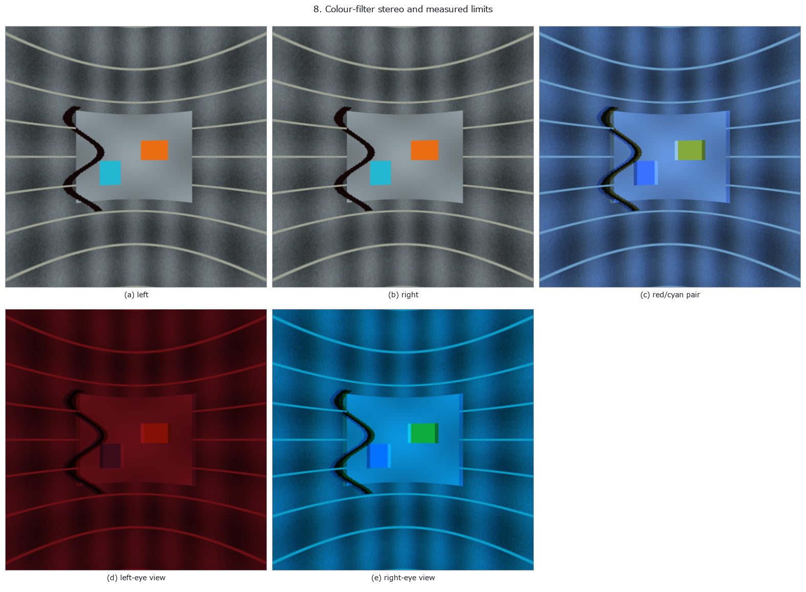
↑ Measurable Omnidirectional Inspection, Stereo Display and Moving Viewports ―― A synthetic 3 m-radius tunnel is captured by two fisheyes and stitched back to a panorama: measured seam error 0.01569 and 0.000 percent blind pixels. The same scene checks solid-angle weighting, moving viewports, 16 of 32 requested tiles, spherical stereo that recovers 3 m as 3.000000 m, rotation correction that raises WS-PSNR from 20.13 to 33.51 dB, cylindrical defect unwrapping, and an actual red/cyan pair. Ideal filters have zero leakage; 10 percent leakage measures 0.0693/0.0014 for the two eyes. On-screen parallax is 1.80 mm. Eight chapters, eight figures, and a 30-frame video. No learning and no calibration.

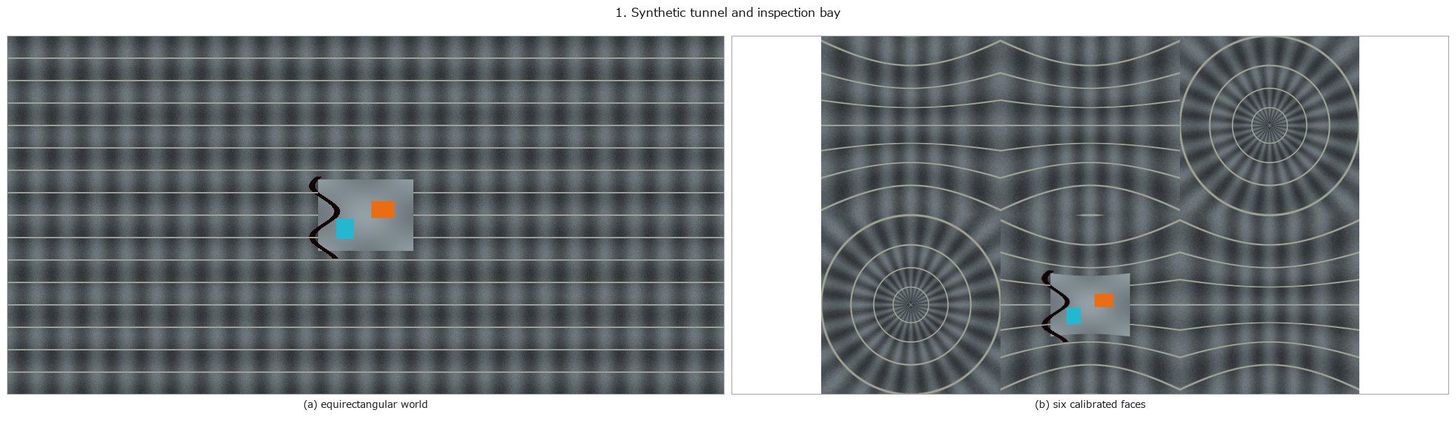
↑ The measurement ―― Seed 275; tunnel radius 3.00 m; crack angular width 3.00 deg. (figure labels are in Japanese; the numbers are the same)

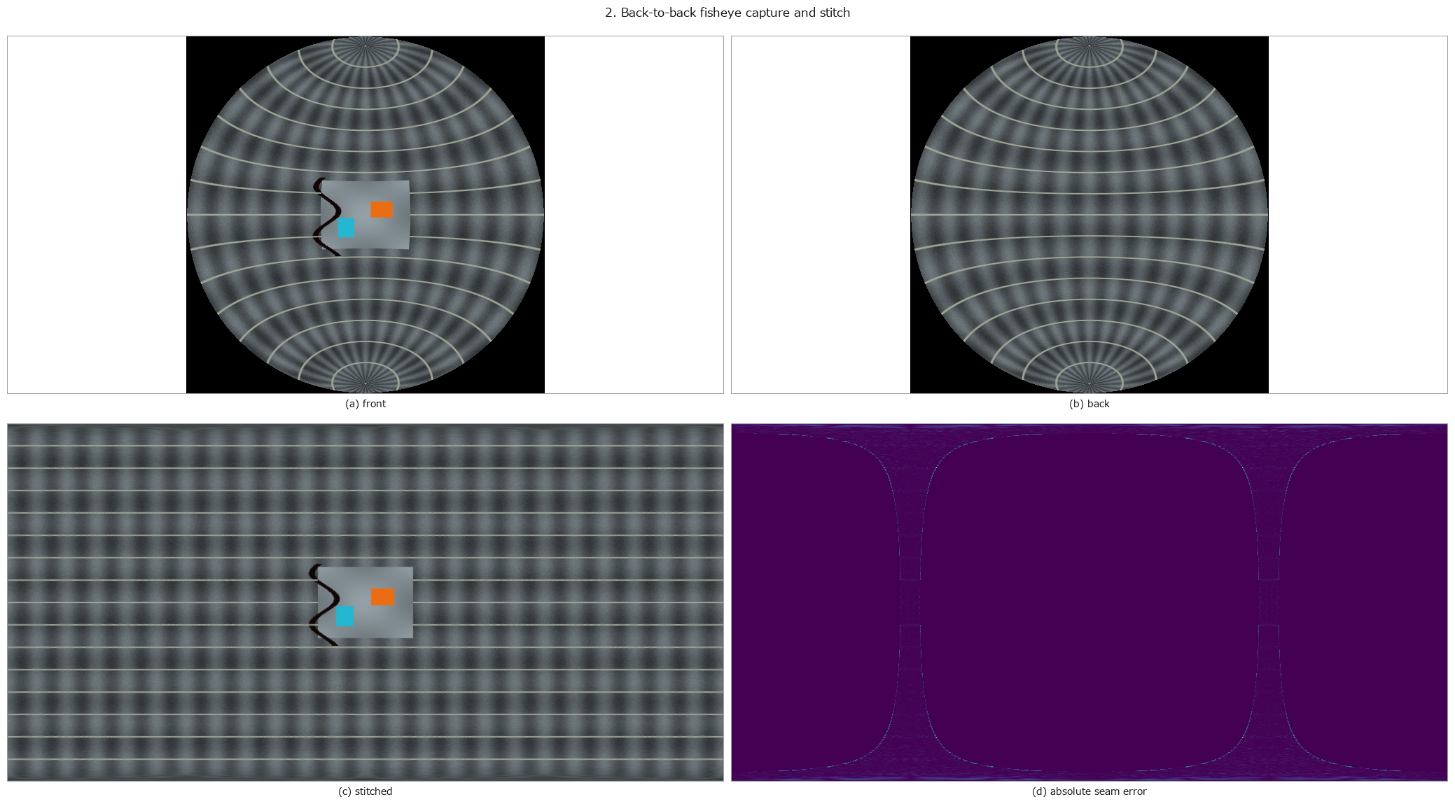
↑ Measured seam MAE 0.0157; blind pixels 0.000 % (reported, never filled silently).

↑ Horizontal half-height width ratio 0.314; defect solid angle 0.03687 sr versus unweighted 0.02399 sr.

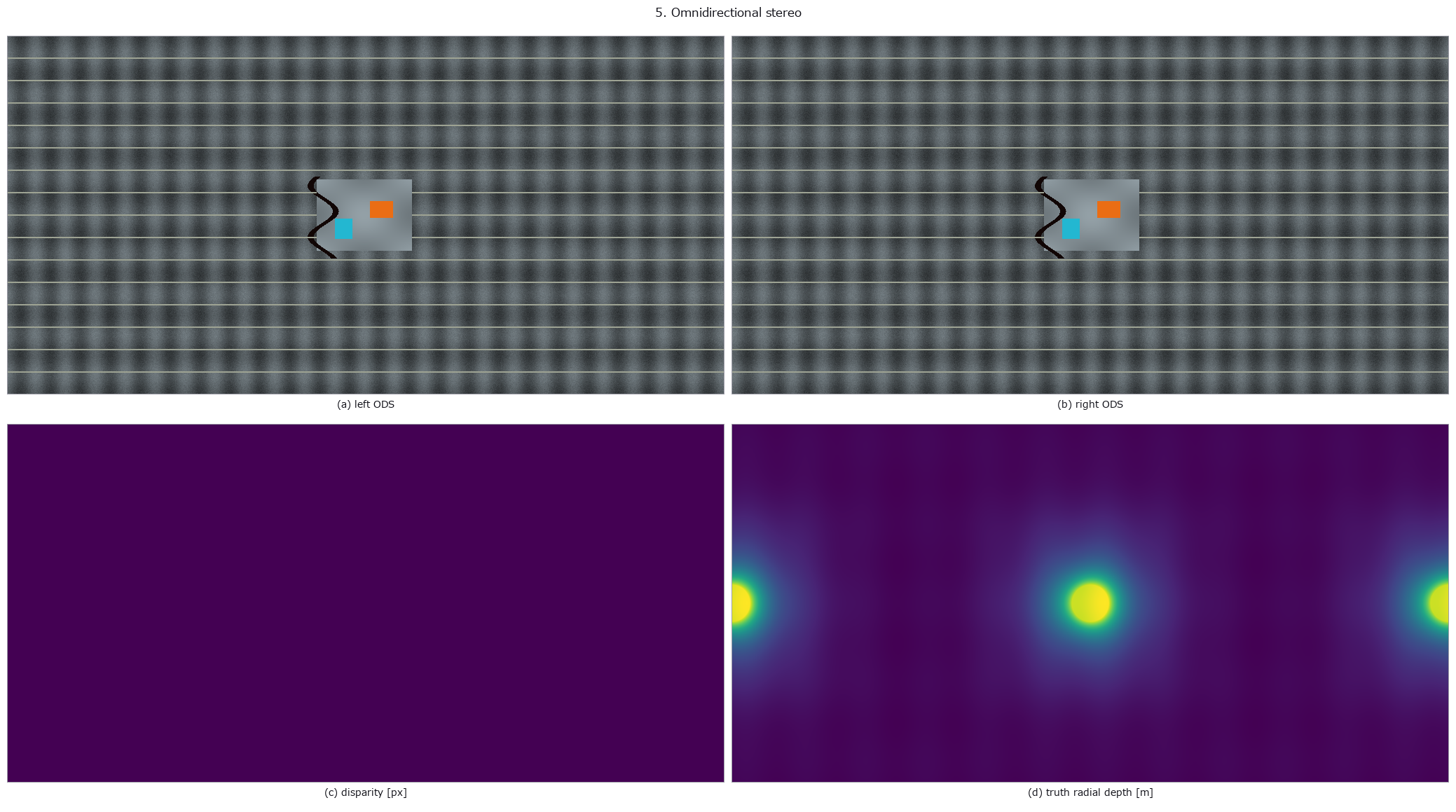
↑ At 3.00 m: disparity 3.477 px and inverted depth 3.000000 m.

↑ WS-PSNR improved from 20.13 to 33.51 dB; residual 0.0078.

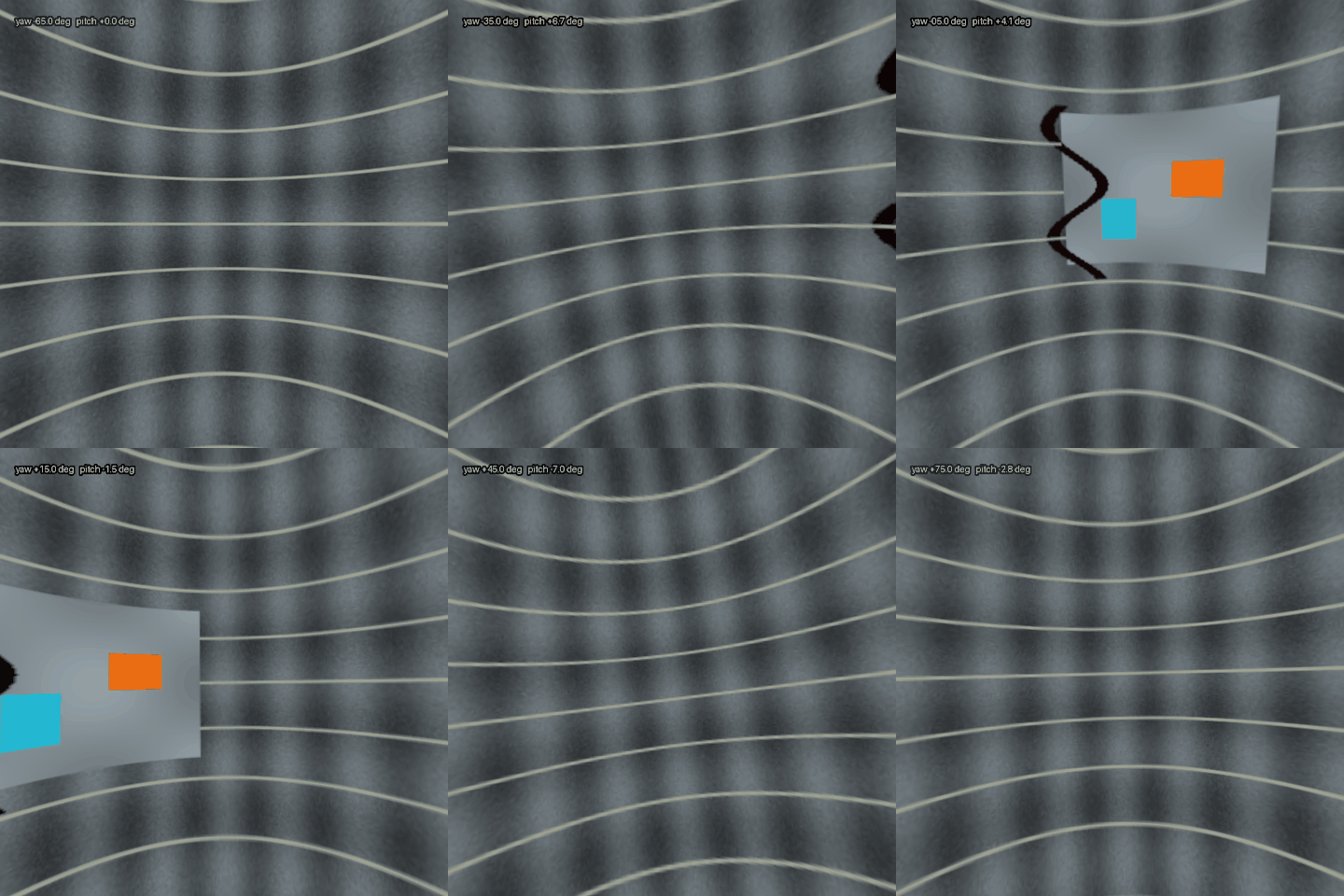
↑ The animation ―― Thirty differing frames; the first frame is already moving.

py -3.11 examples/poc_omni360_inspection.py

Source: examples/poc_omni360_inspection.py

This run produced 9 figures in total - see them all

Ops used (notes): anaglyph_crosstalk · equirect_defect_unwrap_pipe · equirect_filter_gaussian · equirect_from_fisheye_pair · equirect_rotate · equirect_stabilize · equirect_weight_map · ods_depth_to_disparity · ods_disparity_to_depth · omni_anaglyph_compose · stereo_parallax_budget · video360_tile_coverage · video360_viewport_track · viewport_from_equirect · ws_psnr

---

This museum was built together with Claude Code. I set the questions and the direction; Claude Code did the implementation, the sweeps, the control groups and the adversarial checks. That division of labour is what made it possible to run 53 PoCs and collect their figures in two days. If you want to try it, this invitation link gives you a one-week free trial: claude.ai/referral/0sqPw8E_lw

If even one exhibit was worth your time, a like or a stock helps: the reactions decide which wing grows next, so tell me in the comments which measurement from your own field you would want to see. And if you swapped in real data and the cliff moved, that is the story I most want to hear.