【配送最適化入門】焼きなまし法（SA）で局所最適を脱出⑤

この記事について

前回までは局所探索（2-opt・3-opt・LK法）を説明しました。これらはすべて「今より悪くなる方向には進まない」手法です。
そのため局所最適（これ以上改善できない、でも最適解ではない状態）に陥ると、そこから脱出できません。

今回は「あえて悪化を許容することで局所最適から脱出する」焼きなまし法（Simulated Annealing：SA） を説明します。

配送最適化入門シリーズの記事一覧はこちら。

記事	内容
⓪	配送最適化とは？基礎概念
①	近傍法の説明
②	2-optの説明
③	3-optの説明
④	Lin-Kernighan法の説明
⑤（本記事）	焼きなまし法（SA）の説明
⑥	遺伝的アルゴリズム（GA）の説明
⑦	VRPとは？
⑧	VRPをアルゴリズムで解く

焼きなまし法とは？

焼きなまし法は、金属の焼きなまし（徐々に冷やすことで結晶構造を最適化する工程）にヒントを得たメタヒューリスティクスです。

温度（Temperature）が高いうちは悪化も許容する。温度が下がるにつれて、徐々に改善のみを受け入れるようになる。

これにより、探索初期は広く大胆に探索し、後半は精緻に収束していくことができます。

受理確率

現在の解のコストが $C_{current}$、新しい解のコストが $C_{new}$ のとき：

• $C_{new} < C_{current}$（改善）→ 必ず受理
• $C_{new} \geq C_{current}$（悪化）→ 以下の確率で受理

P(\text{受理}) = \exp\!\left(-\frac{C_{new} - C_{current}}{T}\right)

ここで $T$ は現在の温度です。温度が高いほど悪化を受け入れやすく、温度が下がるほど悪化を受け入れなくなります。

冷却スケジュール（Cooling Schedule）

温度をどう下げるかがSAの性能を左右する最も重要なパラメータです。代表的な冷却スケジュールは以下のとおりです。

スケジュール	更新式	特徴
指数冷却	$T_{k+1} = \alpha \cdot T_k$（$\alpha < 1$）	シンプルで最もよく使われる
線形冷却	$T_{k+1} = T_k - \Delta T$	実装は簡単だが収束が早すぎることも
対数冷却	$T_k = T_0 / \log(1 + k)$	理論的な収束保証あり（非常に遅い）

Python実装

import numpy as np
import matplotlib
import matplotlib.pyplot as plt
plt.rcParams['font.family'] = 'Yu Gothic'

def simulated_annealing(route, dist,
                        T_init=1000.0,
                        T_min=1e-3,
                        alpha=0.995,
                        max_iter=100000):
    """
    焼きなまし法によるTSP改善
    route   : 初期ルート
    dist    : 距離行列
    T_init  : 初期温度
    T_min   : 終了温度
    alpha   : 冷却率（指数冷却）
    max_iter: 最大反復回数
    """
    n = len(route)
    current = route[:]
    current_cost = sum(dist[current[i]][current[(i + 1) % n]] for i in range(n))

    best = current[:]
    best_cost = current_cost

    T = T_init
    history = []

    for iteration in range(max_iter):
        if T < T_min:
            break

        # 近傍解の生成：ランダムに2都市を選んでセグメントを反転（2-optムーブ）
        i = np.random.randint(1, n - 1)
        j = np.random.randint(i + 1, n)
        neighbor = current[:]
        neighbor[i:j + 1] = neighbor[i:j + 1][::-1]

        # コスト差を計算
        a, b = current[i - 1], current[i]
        c, d = current[j], current[(j + 1) % n]
        delta = (dist[a][neighbor[i]] + dist[neighbor[j]][d]
                 - dist[a][b] - dist[c][d])

        # 受理判定
        if delta < 0 or np.random.rand() < np.exp(-delta / T):
            current = neighbor
            current_cost += delta

            # 最良解の更新
            if current_cost < best_cost - 1e-10:
                best = current[:]
                best_cost = current_cost

        # 冷却
        T *= alpha
        history.append(current_cost)

    return best, best_cost, history

実行してみる

def generate_cities(n=20, seed=42):
    np.random.seed(seed)
    return np.random.rand(n, 2) * 100

def calc_distance(cities):
    n = len(cities)
    dist = np.zeros((n, n))
    for i in range(n):
        for j in range(n):
            dist[i][j] = np.linalg.norm(cities[i] - cities[j])
    return dist

def total_distance(route, dist):
    n = len(route)
    return sum(dist[route[i]][route[(i + 1) % n]] for i in range(n))

def nearest_neighbor(dist, start=0):
    n = len(dist)
    unvisited = set(range(n))
    route = [start]
    unvisited.remove(start)
    while unvisited:
        current = route[-1]
        nearest = min(unvisited, key=lambda city: dist[current][city])
        route.append(nearest)
        unvisited.remove(nearest)
    return route

cities = generate_cities(n=20, seed=42)
dist   = calc_distance(cities)

# 近傍法で初期解を作成してSAで改善
nn_route = nearest_neighbor(dist, start=7)
sa_route, sa_dist, history = simulated_annealing(
    nn_route, dist,
    T_init=500.0,
    alpha=0.998,
    max_iter=200000
)

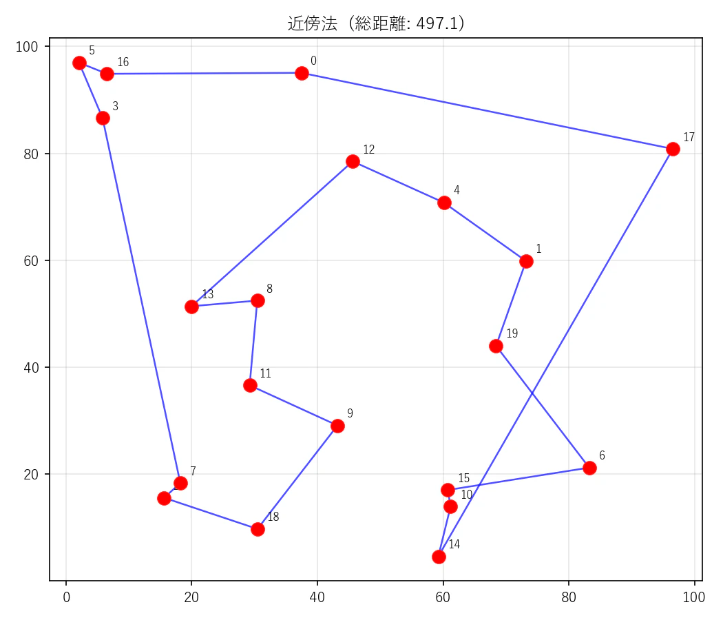
print(f'近傍法:    {total_distance(nn_route, dist):.1f}')
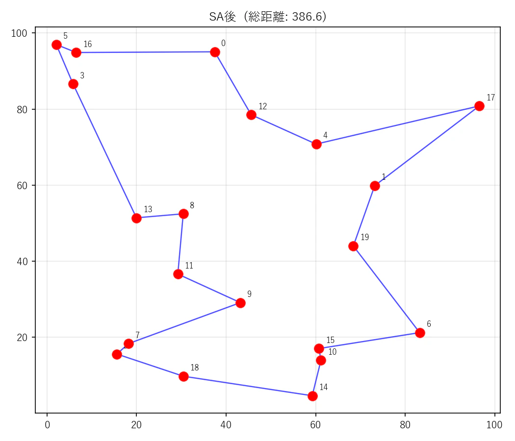
print(f'SA後:      {sa_dist:.1f}')
print(f'改善率:    {(total_distance(nn_route, dist) - sa_dist) / total_distance(nn_route, dist) * 100:.1f}%')

近傍法:    497.1
SA後:      386.6
改善率:    22.2%

コスト履歴の可視化

焼きなまし法の各反復で保持する現在の解のコストを出力すると以下のようになります。

plt.figure(figsize=(8, 4))
plt.plot(history, linewidth=0.5, alpha=0.7)
plt.xlabel('反復回数', fontsize=12)
plt.ylabel('総距離', fontsize=12)
plt.title('焼きなまし法のコスト推移')
plt.grid(True, alpha=0.3)
plt.tight_layout()
plt.savefig('sa_history.png', dpi=150)
plt.show()

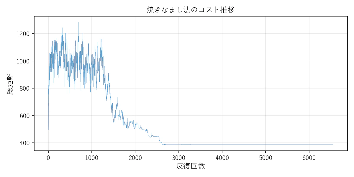
解の悪化も許容しながら、最終的により良い解に収束していくことがわかると思います。

パラメータのチューニング

SAの性能は初期温度・冷却率・反復回数の設定に強く依存します。

初期温度の決め方

初期温度が高すぎると、最初から悪化を受け入れすぎてランダムウォークに近くなってしまいます。
経験的には「初期状態で80〜90%程度の悪化を受け入れる温度」が良いとされています。

def estimate_initial_temperature(route, dist, n_samples=1000, accept_rate=0.8):
    """
    初期温度の推定：悪化の平均コスト差から逆算
    """
    n = len(route)
    deltas = []
    for _ in range(n_samples):
        i = np.random.randint(1, n - 1)
        j = np.random.randint(i + 1, n)
        # 2-optムーブのコスト差
        a, b = route[i - 1], route[i]
        c, d = route[j], route[(j + 1) % n]
        neighbor = route[:]
        neighbor[i:j + 1] = neighbor[i:j + 1][::-1]
        delta = (dist[a][neighbor[i]] + dist[neighbor[j]][d]
                 - dist[a][b] - dist[c][d])
        if delta > 0:
            deltas.append(delta)
    avg_delta = np.mean(deltas) if deltas else 1.0
    # exp(-avg_delta / T) = accept_rate より
    T_init = -avg_delta / np.log(accept_rate)
    return T_init

T_init = estimate_initial_temperature(nn_route, dist)
print(f'推定初期温度: {T_init:.1f}')

まとめ

今回は焼きなまし法を説明しました。

• 焼きなまし法：温度パラメータで悪化を確率的に許容し、局所最適から脱出する
• 受理確率は $\exp(-\Delta C / T)$：温度が高いほど悪化を受け入れやすい
• 冷却スケジュール（特に冷却率 $\alpha$）がSAの性能に最も影響する
• 初期温度は「80〜90%の悪化を受け入れる温度」を目安に設定する

次回は複数の解を同時に進化させる遺伝的アルゴリズム（GA） を説明します。

参考にした記事や本、論文等

• S. Kirkpatrick, C. D. Gelatt, and M. P. Vecchi, "Optimization by Simulated Annealing," Science, vol. 220, pp. 671-680, 1983.
• 焼きなまし法 - Wikipedia