社内勉強会：AWS DeepRacer応用編（モデルの分析・可視化）を開催した

はじめに

社内でAWS DeepRacer人口が増えてきており、もっと自分のモデルを分析したい人向けにAWS DeepRacer勉強会応用編を開催したのでその内容を公開します。

本記事ではモデルの分析・可視化について、AWSから提供されているAWS DeepRacerのログ分析ツールを使用しています。

また、関連記事として以下の記事も参考にしてください。

• AWS DeepRacerのログ分析ツールを使ってみた
• AWS DeepRacer Tokyo Summitリーグ表彰台3名のモデルをログ分析ツールにかけてみた
• 社内勉強会：AWS DeepRacer基礎編（モデル作成）を開催した
• 社内勉強会：AWS DeepRacer基礎編（ログ取得）を開催した
• 社内勉強会：AWS DeepRacer基礎編（ハイパーパラメータ）を開催した

注意点

• 準備の項目がない章は、ノートブックを上から実行してください。
• 準備の項目がある章は、準備の内容と照らし合わせながら、ノートブックを実行してください。
• プログラムが長く、補足コメントがあるものに関しては、折りたたみ表示にしています。

導入手順

SageMaker上のノートブック環境の整備、パッケージインストールの手順については、AWS DeepRacerのログ分析ツールを使ってみた>導入手順をご確認ください。

※ パッケージのインストールについて、SageMakerのノートブックインスタンスを停止して起動すると再度インストールする必要があります。

分析対象のモデル

本記事では、以下の条件で学習したモデルを使⽤しています。

• Reward function：Prevent zig-zagベース
• Action space

Action number	Steering	Speed
0	-25	3
1	-25	6
2	0	3
3	0	6
4	25	3
5	25	6

• Hyperparameter
  • Gradient descent batch size：128
  • その他：デフォルト
• 学習時間：2時間

用語について

分析する上で以下の用語の定義を理解しておくことが重要になります。

• エピソード：1回の学習の中で⽣成される訓練データ
• イテレーション：1回の学習のことだと考えてよいと思います

詳しくはAWS DeepRacer基本概念と用語をご確認ください。

モデルの分析・可視化

では、AWS DeepRacerのログ分析ツールを使用したモデルの分析・可視化について解説していきます。

Requirements

ライブラリ等の読み込みを行います。

セルを実行してエラーとなる場合は、conda_tensorflow_p36にパッケージがインストールされていないことが原因と考えられます。
AWS DeepRacerのログ分析ツールを使ってみた>導入手順を参考にパッケージをインストールしてください。

Download the desired log file given the simulation ID

トレーニング時のシミュレーションIDを使⽤してログファイルをダウンロードします。

準備

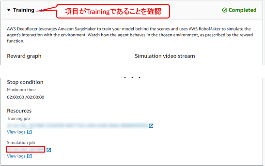
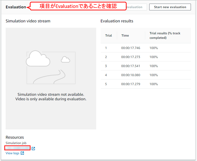
stream_nameにトレーニング時のシミュレーションジョブID（AWS DeepRacerコンソールから確認できます）を設定します。

stream_name = 'sim-abcdefg12345' ## ★トレーニング時のシミュレーションジョブIDを設定
fname = 'logs/deepracer-%s.log' %stream_name

※ AWS DeepRacerコンソールの以下の場所から、トレーニング時のシミュレーションジョブIDを確認できます。

Load waypoints for the track you want to run analysis on

分析に使用するトラックのwaypointsを読み込みます。

準備

get_track_waypointsの引数を使⽤したいトラック名に変更します。

def get_track_waypoints(track_name):
    return np.load("tracks/%s.npy" % track_name)

waypoints = get_track_waypoints("reinvent_base") # ★引数に使用したいトラックを指定
waypoints.shape

※トラックの指定の仕方の例

• 【例1】re:Inventのトラックを使⽤したい場合

waypoints = get_track_waypoints("reinvent_base") # ★引数に使用したいトラックを指定

• 【例2】London Loopのトラックを使⽤したい場合

waypoints = get_track_waypoints("London_Loop_Train") # ★引数に使用したいトラックを指定

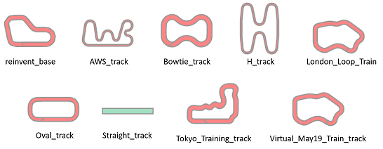
※ 使⽤可能なトラックは以下のコマンドで確認できます。 現在9種類のトラックが使⽤可能です。(2019年7⽉12⽇時点)

!ls tracks/

AWS_track.npy
Bowtie_track.npy
H_track.npy
London_Loop_Train.npy
Oval_track.npy
Straight_track.npy
Tokyo_Training_track.npy
Virtual_May19_Train_track.npy
reinvent_base.npy

Visualize the Track and Waypoints

読み込んだwaypointsからトラックを描画します。

実行結果

全てのトラックを描画した結果は以下のようになります。

Helper Functions

以下の関数を読み込みます。

plot_track：トラックをプロットする関数

def plot_track(df, track_size=(500, 800), x_offset=0, y_offset=0): 
    '''
    Each track may have a diff track size, 
    For reinvent track, use track_size=(500, 800)
    Tokyo, track_size=(700, 1000)
    x_offset, y_offset is used to convert to the 0,0 coordinate system
    '''
    track = np.zeros(track_size) # lets magnify the track by *100 #トラック配列の作成
    for index, row in df.iterrows(): #dfの行数文繰り返し
        x = int(row["x"]) + x_offset #初期座標(0,0)に合わせる修正処理
        y = int(row["y"]) + y_offset #初期座標(0,0)に合わせる修正処理
        reward = row["reward"] 

        track[y,x] = reward #報酬のセット

    fig = plt.figure(1, figsize=(12, 16)) #figureの作成(図の作成)
    ax = fig.add_subplot(111) #axesの作成(軸の作成)
    print_border(ax, center_line, inner_border, outer_border) #トラックコース描画
    return track

plot_top_laps：各エピソードの中で報酬の合計が高いエピソードの軌跡をプロットする関数

def plot_top_laps(sorted_idx, n_laps=5):
    fig = plt.figure(n_laps, figsize=(12, 30)) #figureの作成(図の作成)
    for i in range(n_laps): #表示するプロット分繰り返す
        idx = sorted_idx[i] #各エピソードの中で報酬の合計のトップ順にidxを取得

        episode_data = episode_map[idx] #取得したidxのデータを取得

        ax = fig.add_subplot(n_laps,1,i+1) #axesの作成(軸の作成)

        line = LineString(center_line) 
        plot_coords(ax, line) #中央ラインの点を描画
        plot_line(ax, line) #中央ラインの直線を描画

        line = LineString(inner_border)
        plot_coords(ax, line)  #内側のラインの点を描画
        plot_line(ax, line)  #内側のラインの直線を描画

        line = LineString(outer_border)
        plot_coords(ax, line)  #外側のラインの点を描画
        plot_line(ax, line) #外側のラインの直線を描画


        for idx in range(1, len(episode_data)-1): #エピソードの数分繰り返し
            x1,y1,action,reward,angle,speed = episode_data[idx]
            car_x2, car_y2 = x1 - 0.02, y1 
            plt.plot([x1*100, car_x2*100], [y1*100, car_y2*100], 'b.') #エピソードの座標を描画(座標の点を大きくするために2点描画)

    return fig

Load the training log

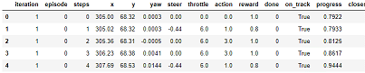
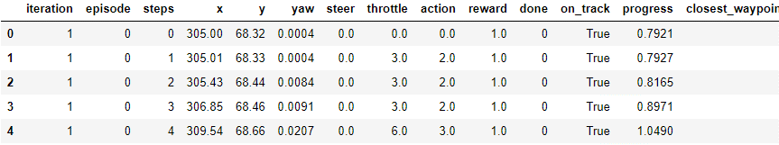
ダウンロードしたログファイルを読み込みます（SIM_TRACE_LOG:を含む行をカンマで分割、項目名を付けてpandasのDataFrameを作成）。

実行結果

補足

データの項目と意味は以下の対応表のようになります。

項目	意味
iteration	イテレーション
episode	エピソード
steps	ステップ数
x, y	車両の座標
yaw	車両の向いている弧度(heading)
steer	ステアリング弧度(steering_angle)
throttle	車両のスピード(speed)
action	アクションリストのインデックス番号
reward	報酬
done	終了したか
on_track	コース上にいるか
progress	コースの消化状況
closest_waypoint	車両の座標から近いwaypointのインデックス※
track_len	トラックの長さ
timestamp	タイムスタンプ

Plot rewards per Iteration

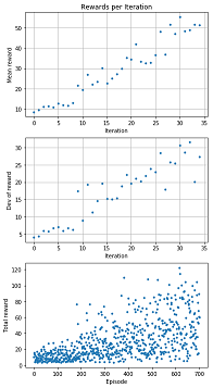
イテレーション毎の報酬の平均・標準偏差を算出しグラフに描画します。

Plot rewards per Iteration

REWARD_THRESHOLD = 100 # ★ 赤で強調させたい閾値を設定

# reward graph per episode
# イテレーション毎の報酬のグラフ

min_episodes = np.min(df['episode'])
max_episodes = np.max(df['episode'])
print('Number of episodes = ', max_episodes)

# イテレーション毎の合計報酬のリストを作成
total_reward_per_episode = list()
for epi in range(min_episodes, max_episodes):
    df_slice = df[df['episode'] == epi]
    total_reward_per_episode.append(np.sum(df_slice['reward']))

# イテレーション毎の報酬の平均用の空のリストを作成
average_reward_per_iteration = list()

# イテレーション毎の報酬の標準偏差用の空のリストを作成
deviation_reward_per_iteration = list()

# イテレーション毎の報酬の平均・標準偏差を算出
buffer_rew = list()
for val in total_reward_per_episode:
    buffer_rew.append(val)

    if len(buffer_rew) == 20: # ★ 平均・標準偏差で扱いたいエピソード数を設定
        average_reward_per_iteration.append(np.mean(buffer_rew))  # 平均を算出
        deviation_reward_per_iteration.append(np.std(buffer_rew)) # 標準偏差を算出
        # reset
        buffer_rew = list()
# 以下描画用

実行結果

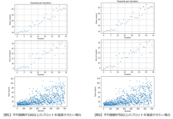
グラフの見方

• 1つ目のグラフ

  • 内容：イテレーション毎の報酬の平均をプロットしています。
  • 横軸：イテレーション
  • 縦軸：報酬の平均

• 2つ目のグラフ

  • 内容：イテレーション毎の報酬の標準偏差をプロットしています。
  • 横軸：イテレーション
  • 縦軸：報酬の標準偏差

• 3つ目のグラフ

  • 内容：エピソード毎の合計報酬をプロットしています。
  • 横軸：エピソード
  • 縦軸：合計報酬

補足

平均報酬が閾値以上のプロットを強調するには、REWARD_THRESHOLDの値を指定します。

• 【例1】平均報酬が100以上のプロットを強調させたい場合

REWARD_THRESHOLD = 100 # ★ 赤で強調させたい閾値を設定

• 【例2】平均報酬が50以上のプロットを強調させたい場合

REWARD_THRESHOLD = 50 # ★ 赤で強調させたい閾値を設定

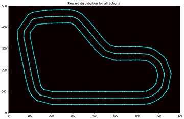
Analyze the reward distribution for your reward function

設定した報酬関数によって報酬の分布がどのようになっているのか視覚的に分かりやすく分析します。

実行結果

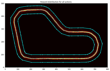
グラフの見方

以下の図のようなカラーマップを使用しています。

また、グラフのセンターライン付近を拡大すると以下の図のようになります。

センターラインに近づくに従い、高い報酬が与えられていることがわかります。

補足

以下のプログラムの、plt.imshowのcmapの値を変更することでカラーマップの設定した色に変更可能です。
参考）Choosing Colormaps in Matplotlib

track = plot_track(df)
plt.title("Reward distribution for all actions ")
im = plt.imshow(track, cmap='hot', interpolation='bilinear', origin="lower") # ★cmapの中の設定を変更することでカラーマップの設定した色に変更可能

Plot a particular iteration

指定したiterationの通過した分布を表示します。

準備

描画したいイテレーションIDをiteration_idに設定します。

iteration_id = 30 # ★描画したいイテレーションIDに変更
track = plot_track(df[df['iteration'] == iteration_id])
plt.title("Reward distribution for all actions ")
im = plt.imshow(track, cmap='hot', interpolation='bilinear', origin="lower") 

実行結果

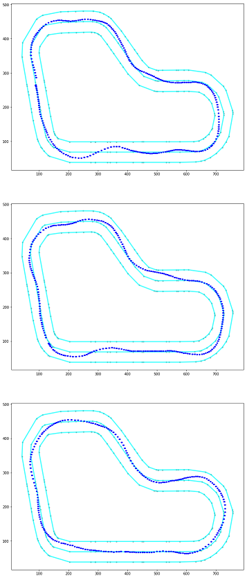
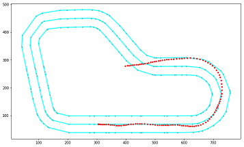
Path taken for top reward iterations

エピソード毎の報酬合計の上位3位までのエピソードの軌跡を確認できます。

実行結果

Path taken in a particular episode

指定したエピソードの軌跡を確認することが出来ます。

準備

以下のプログラムの、plot_episode_runのEの値を変更することで、描画したいエピソードを指定することができます。

fig=plt.figure(1, figsize=(12, 16))
plot_episode_run(df, E=500, ax=fig.add_subplot(211)) # ★Eの値にエピソードIDを指定

実行結果

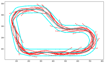
Path taken in a particular Iteration

指定したイテレーションの中の全てのエピソードの軌跡を確認することができます。

準備

以下のプログラムの、iteration_idの値を変更することで、イテレーションを指定することができます。

iteration_id = 20 # ★イテレーションIDを指定
fig = plt.figure(1, figsize=(12, 16))
ax = fig.add_subplot(211)
for i in range((iteration_id-1)*EPISODE_PER_ITER, (iteration_id)*EPISODE_PER_ITER):
    plot_episode_run(df, E=i, ax=ax)

実行結果

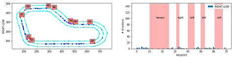
Action breakdown per iteration and historgram for action distribution for each of the turns - reinvent track

このプログラムでは、指定したイテレーションについて、どのコースの区間（waypointの区間）でどのアクションが使われているかを分析します。

Action breakdown per iteration and historgram for action distribution for each of the turns - reinvent track

iteration_id = [20] # ★分析したいイテレーションIDを指定

fig = plt.figure(figsize=(16, 24))
iterations_downselect = iteration_id

# Track Segment Labels
# Trackのセグメントラベルの設定

action_names = ['RIGHT-LOW', 'RIGHT-HIGH', 'STRAIGHT-LOW', 'STRAIGHT-HIGH', 'LEFT-LOW', 'LEFT-HIGH'] # ★アクションスペースに合う名前を指定
vert_lines = [10,25,32,33,40,45,50,53,61,67] # 左図 赤四角の数字描画用
track_segments = [(15, 100, 'hairpin'),      # 右図 テキスト表示用
                  (32, 100, 'right'),
                  (42, 100, 'left'),
                  (51, 100, 'left'),
                  (63, 100, 'left')]

# 右図 エラーボックス描画用
segment_x = np.array([15, 32, 42, 51, 63])
segment_y = np.array([0, 0, 0, 0, 0])

segment_xerr = np.array([[5, 1, 2, 1, 2], [10, 1, 3, 2, 4]])
segment_yerr = np.array([[0, 0, 0, 0, 0], [150, 150, 150, 150, 150]])

wpts_array = center_line 

# イテレーションごとに描画
for iter_num in iterations_downselect:

    # Slice the data frame to get all episodes in that iteration
    # 指定したイテレーションのデータのみを抽出する
    df_iter = df[(iter_num == df['iteration'])]
    n_steps_in_iter = len(df_iter)
    print('Number of steps in iteration=', n_steps_in_iter)

    th = 0.8 # ★ 描画したい報酬の閾値を指定する
    # アクション数ごとに描画
    for idx in range(len(action_names)):
        ax = fig.add_subplot(6, 2, 2*idx+1)
        print_border(ax, center_line, inner_border, outer_border)

        # 閾値以上の報酬で該当するアクションのデータを抽出
        df_slice = df_iter[df_iter['reward'] >= th]
        df_slice = df_slice[df_slice['action'] == idx]

        ax.plot(df_slice['x'], df_slice['y'], 'b.')  # 左図に●をプロット

        # 左図に赤四角のwaypointを描画
        for idWp in vert_lines:
            ax.text(wpts_array[idWp][0], wpts_array[idWp][1]+20, str(idWp), bbox=dict(facecolor='red', alpha=0.5))

        #ax.set_title(str(log_name_id) + '-' + str(iter_num) + ' w rew >= '+str(th))
        ax.set_ylabel(action_names[idx])   # 左図のY軸ラベルを描画

        # calculate action way point distribution
        # waypointに含まれるアクションの分布を算出
        action_waypoint_distribution = list()
        for idWp in range(len(wpts_array)):
            action_waypoint_distribution.append(len(df_slice[df_slice['closest_waypoint'] == idWp]))
# 以下描画用

準備

イテレーションIDの指定の仕方

iteration_idに分析したいイテレーションを指定します。

iteration_id = [20] # ★分析したいイテレーションIDを指定

アクションの指定の仕方

モデルによってアクション数が異なるので、自身のモデルのアクションに対応するように、action_namesを修正する必要があります。

今回はSteering angle granularity：3、Speed arnularity：2の6段階のモデルを対象としているので、サイズ6の配列を使用しています。配列の1番目がAction number 0～6番目がAction number5に対応するように指定します。

• 【例1】Steering angle granularity：3、Speed arnularity：2の6段階のモデルの場合

action_names = ['RIGHT-LOW', 'RIGHT-HIGH', 'STRAIGHT-LOW', 'STRAIGHT-HIGH', 'LEFT-LOW', 'LEFT-HIGH'] # ★アクションスペースに合う名前を指定

• 【例2】Steering angle granularity：3、Speed arnularity：1の3段階のモデルの場合

action_names = ['RIGHT', 'STRAIGHT', 'LEFT'] # ★アクションスペースに合う名前を指定

描画したい報酬の閾値の設定の仕方

thに閾値の値を指定します。

• 【例1】閾値を0.8にする場合

th = 0.8 # ★ 描画したい報酬の閾値を指定する

• 【例2】閾値を0.3にする場合

th = 0.3 # ★ 描画したい報酬の閾値を指定する

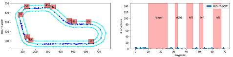
実行結果

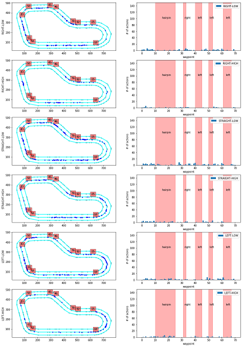
グラフの見方

• 左のグラフ

  • 内容：コース上で該当するアクションが使われた場所をプロットしています。
  • 赤四角の数字：その場所に該当するwaypointの番号

• 右のグラフ

  • 内容：waypointの区間で該当するアクションが使われた回数を示しています。
  • 横軸：waypoint
  • 縦軸：アクション数

• 縦方向のグラフの違い

  • 上からアクションスペースが「'RIGHT-LOW', 'RIGHT-HIGH', 'STRAIGHT-LOW', 'STRAIGHT-HIGH', 'LEFT-LOW', 'LEFT-HIGH'」のグラフを示しています。
  • action_names変数に入れた値となります。

Simulation Image Analysis - Probability distribution on decisions (actions)

コース画像に対して、どの程度の信頼度でアクションを選択しているかの分析をしています。

準備

S3 bucketとprefix・ダウンロードするモデルの指定

以下のコマンドを実行するとS3のbucketとprefixが確認できます。

!grep "S3 bucket" $fname
!grep "S3 prefix" $fname

出力されたS3 bucketとS3 prefixの値を以下s3_bucketとs3_prefixにコピーします。
また、--includeの引数の*model_N*のNにダウンロードしたいイテレーション番号を指定します。

※ *model_3*であれば、イテレーションIDが3番と30番台のモデルがダウンロードされます。

s3_bucket = 'aws-deepracer-abcd1234-ab12-cd34-ef56-abcdefg12345' # ★s3 bucketをコピー
s3_prefix = 'DeepRacer-SageMaker-RoboMaker-comm-127356273604-20190612111111-12345678-9999-ab12-cd34-abcdefg12345'# ★s3 prefixをコピー
!aws s3 sync s3://$s3_bucket/$s3_prefix/model/ intermediate_checkpoint/ --exclude "*" --include "*model_3*" # ★ダウンロードしたいイテレーションの番号を指定する

以下のコマンドを実行すると、ダウンロードされたモデルを確認することができます。

!ls $GRAPH_PB_PATH

分析するイテレーションの指定の仕方

ダウンロードされたモデルの中から、分析したいイテレーションIDをiterationsに指定します。

Simulation Image Analysis - Probability distribution on decisions

model_inference = []
iterations = [30, 35] # ★GRAPH_PB_PATHフォルダから分析したいモデルを指定する

# 各モデルに対して、各コース画像に対する推論結果を算出
for ii in iterations:
    model, obs, model_out = load_session(GRAPH_PB_PATH + 'model_%s.pb' % ii)
    arr = []
    # 各コース画像に対する推論を実行
    for f in all_files[:]:
        img = Image.open(f)
        img_arr = np.array(img)
        img_arr = rgb2gray(img_arr)
        img_arr = np.expand_dims(img_arr, axis=2) # 画像ファイルを推論用の形式に変換
        current_state = {"observation": img_arr} #(1, 120, 160, 1)
        y_output = model.run(model_out, feed_dict={obs:[img_arr]})[0]  # コース画像に対する推論を実行
        arr.append (y_output)

    model_inference.append(arr) # 推論結果をappend
    model.close()
    tf.reset_default_graph()

model_inference = []
iterations = [30, 35] # ★GRAPH_PB_PATHフォルダから分析したいモデルの番号を指定する

実行結果

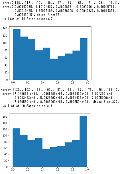
グラフの見方

横軸、縦軸は以下を示しています。

• 横軸：推論結果が高いアクション上位1位と上位2位の差
• 縦軸：カウント

つまり、0.8～1.0あたりが大きいヒストグラムがよく学習できていると考えることができます。

補足

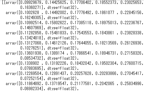
算出方法について

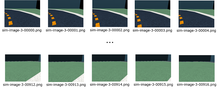
model_inferenceには以下のようなデータが保存されています。これは左からアクションスペース0～5が推論された確率を示しており、推論結果の確率が917枚分（simulation_episodeのフォルダにある画像の枚数）の含まれるリストが2イテレーション分（今回指定したイテレーション数）含まれるリストになっています。

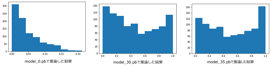
グラフの比較

以下のグラフはイテレーション0、30、35のグラフを示しています。イテレーションが増えるに従い、0.0付近のヒストグラムが減っているので、よく学習できていることがわかります。

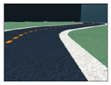
入力値について

推論の入力値として以下のようなコース画像を使用しています。

Model CSV Analysis

モデルのCSVファイルの分析をします。

準備

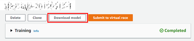
• AWS DeepRacerのコンソール画面からモデルをダウンロードします。

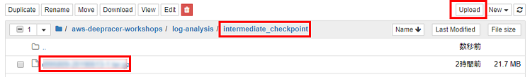
• ダウンロードしたファイルをintermediate_checkpointフォルダにアップロードします。

• 以下のコマンドを実行しtarファイルを解凍します。

!tar xzf intermediate_checkpoint/model_name.tar.gz -C intermediate_checkpoint/ # ★model_nameを自身のモデル名に変更する

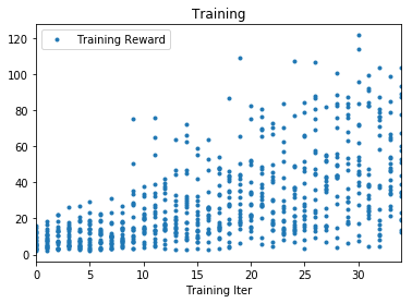
実行結果

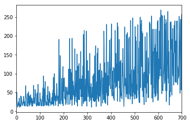
グラフの見方

• 1つ目のグラフ

  • 内容：トレーニングイテレーション毎の報酬を示しています。
  • 横軸：トレーニングイテレーション
  • 縦軸：報酬

• 2つ目のグラフ

  • 内容：エピソード毎のエピソードの長さ（ステップ数）示しています。
  • 横軸：エピソード
  • 縦軸：エピソードの長さ（ステップ数）

Evaluation Run Analyis

評価ログの分析をします。

準備

eval_simにEvaluationに記載されているシミュレーションIDを設定します。

eval_sim = 'sim-abcdefg12345'
eval_fname = './logs/deepracer-eval-%s.log' % eval_sim

実行結果

Grid World Analysis

スピードをエピソード毎の走行経路と一緒に描画します。

準備

N_EPISODESにEvaluation実行時に指定したラップ数を指定します。

N_EPISODES = 3  # ★Evaluation実行時に指定したラップ数を指定する

実行結果

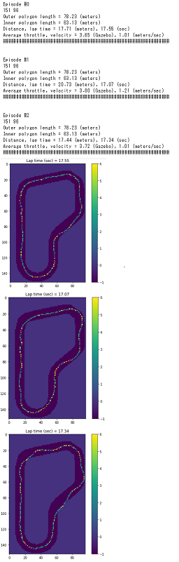
グラフの見方

スピードが速いほど黄色くなっています。
黄色い色が多いほど全体的に高速で走行していると考えられます。

補足

Grid Worldについて

処理としては１ｘ１のグリッド内に存在するスピードの平均値をプロットしているようです。
(0, 0)から(max(x), max(y))まで1ずつ増やしていき、データの中で x-1～x、x-1～yまでの間のスピードの平均値をそのマスの値としているようです。

Distanceについて

走行距離は2つの座標間の距離を計算したものを足し算した結果のようです。

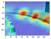
What is the model looking at?

モデルが画像をどのように見ているのかをGrad-CAMという手法を使って可視化します。
Grad-CAM：Gradient-weighted Class ActivationMapping
Grad-CAM:
Visual Explanations from Deep Networks via Gradient-based Localization
PDFを見ていただくと分かりやすいですが、DogやCatという分類結果に強く影響している領域をヒートマップで表現しています。
AWS DeepRacerに置き換えると、特定のアクションスペース（ステアリング角度とスピードの組み合わせ）を選択する場合に強く影響している領域を可視化しているといえます。

What is the model looking at?

import cv2
import numpy as np
import tensorflow as tf

# デフォルトは以下の通りです
# category_index=0 : アクションスペース0のアクションに対する分析になります
# num_of_actions=6 : アクションスペースを6段階で作成したモデルを分析します
def visualize_gradcam_discrete_ppo(sess, rgb_img, category_index=0, num_of_actions=6):
    '''
    @inp: model session, RGB Image - np array, action_index, total number of actions 
    @return: overlayed heatmap
    '''

    img_arr = np.array(rgb_img)
    img_arr = rgb2gray(img_arr)
    img_arr = np.expand_dims(img_arr, axis=2) # img_arr.shape = (120, 160, 1)

    # sess.runまでは準備です

    # 画像データをインプット
    # x に対して入力のテンソルを紐づけ、そのテンソルに対して画像のデータを設定します
    # y に対して
    # get_tensor_by_name で指定する値は下記の中から目的に応じて選択しているようです
    # sess.graph.get_operations()
    x = sess.graph.get_tensor_by_name('main_level/agent/main/online/network_0/observation/observation:0')
    y = sess.graph.get_tensor_by_name('main_level/agent/main/online/network_1/ppo_head_0/policy:0')
    feed_dict = {x:[img_arr]}

    # 出力層を取得します
    #Get he policy head for clipped ppo in coach
    model_out_layer = sess.graph.get_tensor_by_name('main_level/agent/main/online/network_1/ppo_head_0/policy:0')
    # 出力層の中で指定したアクションスペースに対応する部分のみを取り出す
    # multiply: 行列の積
    # 引数1: model_out_layerからは、アクションスペース毎の出力が得られる
    # 引数2: one_hotにより、category_indexで指定したアクションスペースの値以外を0にする
    loss = tf.multiply(model_out_layer, tf.one_hot([category_index], num_of_actions))
    # すべての要素の和を取る loss[0]なのは1次元の配列のため
    reduced_loss = tf.reduce_sum(loss[0])
    conv_output = sess.graph.get_tensor_by_name('main_level/agent/main/online/network_1/observation/Conv2d_4/Conv2D:0')
    # 勾配を計算する
    grads = tf.gradients(reduced_loss, conv_output)[0]
    output, grads_val = sess.run([conv_output, grads], feed_dict=feed_dict)
    # その領域の平均を重みとして計算します
    # grads_val.shape (1, 11, 16, 64)
    weights = np.mean(grads_val, axis=(1, 2)) # (1, 64)
    # 画素値に重みを加えます
    cams = np.sum(weights * output, axis=3)
    # cams :(1, 11, 16) , weights :(1, 64), output :(1, 11, 16, 64) 
    # 11 x 16 の配列要素それぞれに weights * output の要素の合計値が格納される

    ##im_h, im_w = 120, 160##
    im_h, im_w = rgb_img.shape[:2]

    cam = cams[0] #img 0
    image = np.uint8(rgb_img[:, :, ::-1] * 255.0) # RGB -> BGR
    cam = cv2.resize(cam, (im_w, im_h)) # zoom heatmap
    cam = np.maximum(cam, 0) # relu clip 0以上の値にする
    #heatmap = cam / np.max(cam) # normalize
    heatmap = cam / (np.max(cam) + 1E-5) # normalize
    cam = cv2.applyColorMap(np.uint8(255 * heatmap), cv2.COLORMAP_JET) # grayscale to color カラーマップ JETの256段階でヒートマップを表現する
    cam = np.float32(cam) + np.float32(image) # overlay heatmap 元画像にヒートマップを重ねる
    cam = 255 * cam / (np.max(cam) + 1E-5) ##  Add expsilon for stability
    cam = np.uint8(cam)[:, :, ::-1] # to RGB

    return cam

準備

model_pathのmodel_N.pbを分析したいモデルの番号に変更します。

model_path = GRAPH_PB_PATH + 'model_35.pb' # ★分析したいモデルの番号

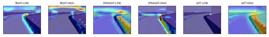
補足

ヒートマップは画像のどのあたりが行動に影響を与えているかを表現していると思われます。
ただし、色が沢山ついているからといって必ずしも実際にとる行動と一致するわけではないようです。
各アクションスペースに対応するヒートマップを表示してみます。

image_idx = 850
num_of_actions = 6

heatmaps = []
model_path = GRAPH_PB_PATH + 'model_35.pb' #Change this to your model 'pb' frozen graph file
model, obs, model_out = load_session(model_path)

for f in all_files[image_idx:image_idx+1]:
    img = np.array(Image.open(f))
    for idx in range(num_of_actions):
        heatmap = visualize_gradcam_discrete_ppo(model, img, category_index=idx, num_of_actions=num_of_actions)
        heatmaps.append(heatmap)
tf.reset_default_graph()

fig = plt.figure(figsize=(16, 48))
for i in range(len(heatmaps)):
    ax = fig.add_subplot(1, len(heatmaps), i+1)
    ax.set_title(action_names[i], fontsize=8)
    ax.tick_params(labelbottom=False, labelleft=False)
    plt.xticks([])
    plt.yticks([])
    ax.imshow(heatmaps[i])

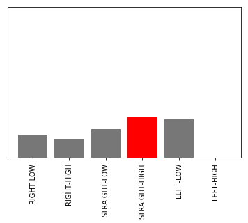
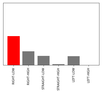
入力画像に対してどのような行動を取る確率が高いかを調べてみます。

# 予測する関数
def predict_for_action_space(sess, rgb_img, num_of_actions=6):

    img_arr = np.array(rgb_img)
    img_arr = rgb2gray(img_arr)
    img_arr = np.expand_dims(img_arr, axis=2)

    x = sess.graph.get_tensor_by_name('main_level/agent/main/online/network_0/observation/observation:0')
    y = sess.graph.get_tensor_by_name('main_level/agent/main/online/network_1/ppo_head_0/policy:0')
    feed_dict = {x:[img_arr]}

    prediction = sess.run(y, feed_dict=feed_dict)
    return prediction

# グラフ化する関数
# https://www.tensorflow.org/tutorials/keras/basic_classification
def plot_value_array(predictions_array, action_labels):
    plt.grid(False)
    plt.xticks([])
    plt.yticks([])
    thisplot = plt.bar(range(len(predictions_array)), predictions_array, color="#777777")
    plt.xticks(range(len(predictions_array)), action_labels, rotation=90)
    plt.ylim([0, 1])
    predicted_label = np.argmax(predictions_array)

    thisplot[predicted_label].set_color('red')

# What is the model looking at?と同じ画像ファイルを読み込む
f = all_files[image_idx]
img = np.array(Image.open(f))

prediction = predict_for_action_space(model, img, num_of_actions=6)

# 下記で定義したラベルを使います
# Action breakdown per iteration and historgram for action distribution for each of the turns - reinvent track
action_names = ['RIGHT-LOW', 'RIGHT-HIGH', 'STRAIGHT-LOW', 'STRAIGHT-HIGH', 'LEFT-LOW', 'LEFT-HIGH']

plot_value_array(prediction[0], action_names)

入力画像

アクションをとる確率

現実の画像に当てはめてみた結果は以下のようになります。

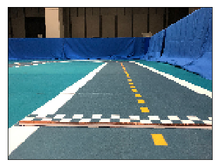
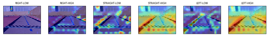
実機の環境では、コースとあまり関係のない、柱の情報がアクションに影響を及ぼしている場合もあるということがわかります。

まとめ

本記事では、モデルの分析・可視化について解説しました。

効率的にスピードアップを図るためにもモデル分析は有効です。
モデルを分析してAWS DeepRacer世界一を目指しましょう。