はじめに

最近トピックモデルを勉強する機会があり，ネット上の記事だけでトピックモデル（今回はLDA）をザックリと理解して，Pythonで簡単に試してみました．
簡単な理解にとどまっているので，間違い，ご指摘等がございましたらコメントを頂けると幸いです．

今回はトピックモデルをPythonで実装して

ニュース記事解析
「小説家になろう」解析

をやってみます．
どちらのテーマにおいても，これまでに試みた方が書かれた多くの記事を参考にさせて頂きました m(__)m

実行環境

mac OS Mojave
Python 3.5.5
gensim 3.4.0
mecab-python3 0.996.2
pyLDAvis 2.1.2

参考記事・文献

トピックモデルについて
Python実装
ニュース記事解析
- WordCloudとpyLDAvisによるLDAの可視化について
「小説家になろう」解析
- 小説家になろうのランキングをトピックモデルで解析(gensim)
- GensimPy3を使って小説家になろうのトピックモデルを解析

トピックモデルとは

今回はトピックモデルの1種であるLDAに着目しました．LDAとは文書がどのようなトピックから，どんな割合で構成されているかを推定するモデルです．
下の画像はLDAの論文内のものです．上側には推定された4つのトピックと，それらトピックに属する単語が，下側は文書内の単語がどのトピックによって構成されているかを表しています．ここから分かるようにLDAでは，文書が1つのトピックから成り立つのではなく，複数のトピックから成り立つと仮定しています．

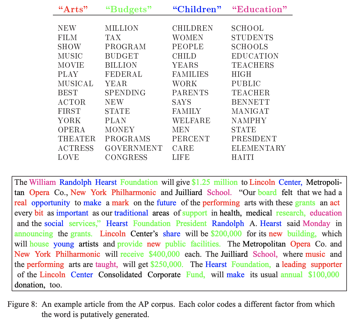
トピックモデルでは，文書ごとのトピックの構成比率「トピック分布」と，トピックごとの単語の比率「単語分布」を推定します．

ニュース記事解析

ここでは主にこの記事内でやられている内容・コードを拝借しました．
livedoorニュースコーパスを利用してLDAを行い，結果の可視化を行います．
参考記事内のものとほぼ同じですが，ソースコードを以下に示します．

ソースコード

必要ライブラリのインポート等

import glob
import numpy as np
from tqdm import tqdm
import math
import MeCab
import urllib
import gensim
import pyLDAvis
import pyLDAvis.gensim
from wordcloud import WordCloud
from PIL import Image
import matplotlib
import matplotlib.pylab as plt

np.random.seed(0)
FONT = "/Library/Fonts/Arial Unicode.ttf"

ニュース記事のパスと形態素解析用のストップワードの定義

# paths to textss
text_paths = glob.glob('./livedoor-news-corpus/text/**/*.txt')

# define stop words
req = urllib.request.Request('http://svn.sourceforge.jp/svnroot/slothlib/CSharp/Version1/SlothLib/NLP/Filter/StopWord/word/Japanese.txt')
with urllib.request.urlopen(req) as res:
    stopwords = res.read().decode('utf-8').split('\r\n')
while '' in stopwords:
    stopwords.remove('')

形態素解析用の関数定義

def analyzer(text, mecab, stopwords=[], target_part_of_speech=['proper_noun', 'noun', 'verb', 'adjective']):

    node = mecab.parseToNode(text)
    words = []

    while node:

        features = node.feature.split(',')
        surface = features[6]

        if (surface == '*') or (len(surface) < 2) or (surface in stopwords):
            node = node.next
            continue

        noun_flag = (features[0] == '名詞')
        proper_noun_flag = (features[0] == '名詞') & (features[1] == '固有名詞')
        verb_flag = (features[0] == '動詞') & (features[1] == '自立')
        adjective_flag = (features[0] == '形容詞') & (features[1] == '自立')


        if ('proper_noun' in target_part_of_speech) & proper_noun_flag:
            words.append(surface)
        elif ('noun' in target_part_of_speech) & noun_flag:
            words.append(surface)
        elif ('verb' in target_part_of_speech) & verb_flag:
            words.append(surface)
        elif ('adjective' in target_part_of_speech) & adjective_flag:
            words.append(surface)

        node = node.next

    return words

LDAのための辞書とコーパス作成
登場が3回未満の単語 or 5割以上の文書に登場する単語をフィルタリングしています．

# make dictionary and corpus
mecab = MeCab.Tagger('-d /usr/local/lib/mecab/dic/ipadic')
titles = []
texts = []
for text_path in text_paths:

    text = open(text_path, 'r').read()
    text = text.split('\n')
    title = text[2]
    text = ' '.join(text[3:])
    words = analyzer(text, mecab, stopwords=stopwords, target_part_of_speech=['noun', 'proper_noun'])
    texts.append(words)

dictionary = gensim.corpora.Dictionary(texts)
dictionary.filter_extremes(no_below=3, no_above=0.5)
corpus = [dictionary.doc2bow(t) for t in texts]

LDAの実行とWordCloudによる可視化
まずはトピック数を10としてみます．

# LDA
num_topics = 10
lda_model = gensim.models.ldamodel.LdaModel(corpus=corpus,
                                            id2word=dictionary,
                                            num_topics=num_topics,
                                            random_state=0)

# Visualize
ncols = math.ceil(num_topics/2)
nrows = math.ceil(lda_model.num_topics/ncols)
fig, axs = plt.subplots(ncols=ncols, nrows=nrows, figsize=(15,7))
axs = axs.flatten()

def color_func(word, font_size, position, orientation, random_state, font_path):
    return 'darkturquoise'

for i, t in enumerate(range(lda_model.num_topics)):

    x = dict(lda_model.show_topic(t, 30))
    im = WordCloud(
        font_path=FONT,
        background_color='white',
        color_func=color_func,
        random_state=0
    ).generate_from_frequencies(x)
    axs[i].imshow(im)
    axs[i].axis('off')
    axs[i].set_title('Topic '+str(t))

plt.tight_layout()
plt.savefig("./visualize.png")

pyLDAvisによる可視化

# pyLDAvis
vis = pyLDAvis.gensim.prepare(lda_model, corpus, dictionary, sort_topics=False)
pyLDAvis.save_html(vis, './pyldavis_output.html')

結果

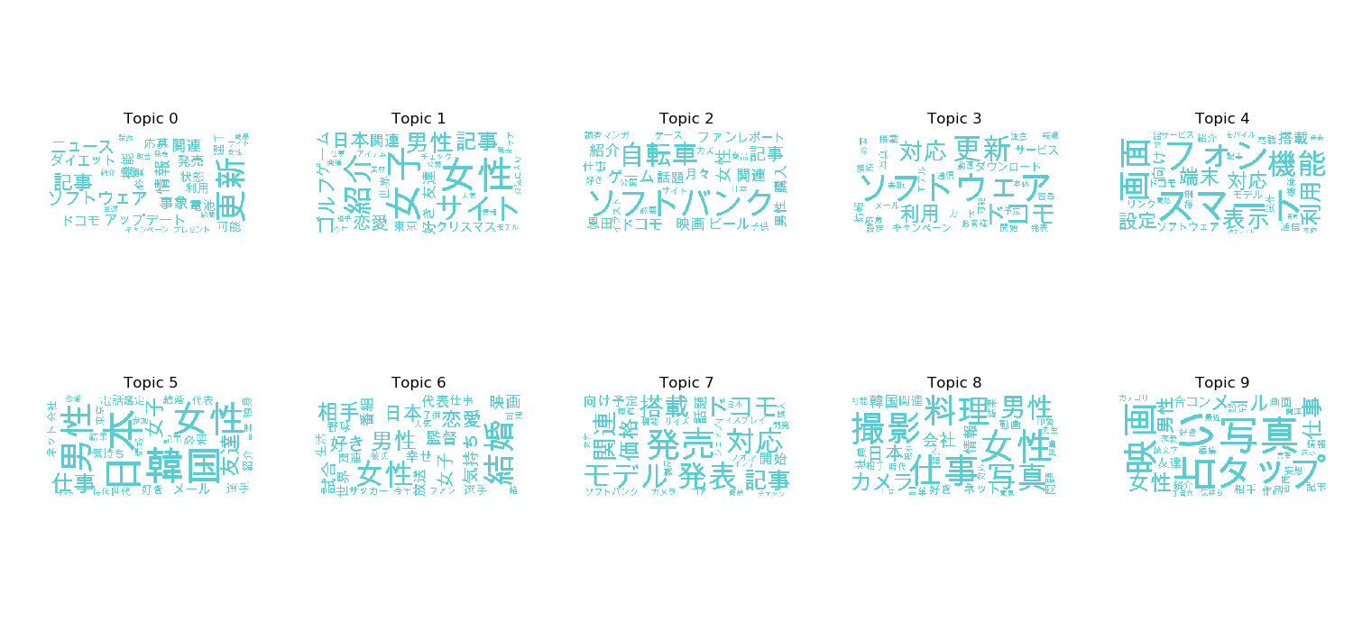
以下はWordCloudによるトピックごとの単語割合の可視化と，pyLDAvisによる可視化結果です．
WordCloudによる可視化結果から，

Topic 4, 7は携帯電話関連
Topic 6は恋愛関連
Topic 8, 9は女性の趣味関連

のトピックであるように思えなくもないです．

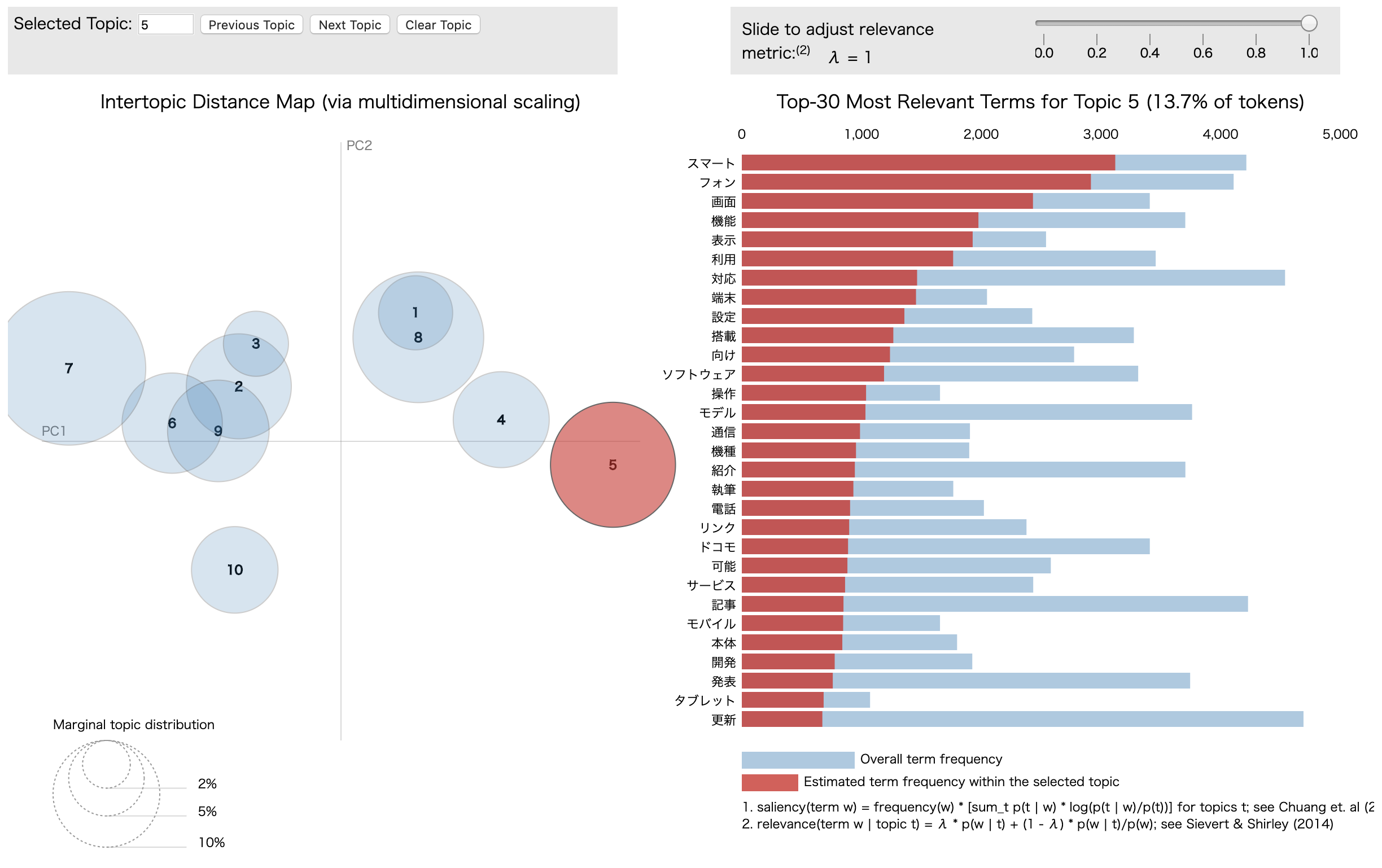
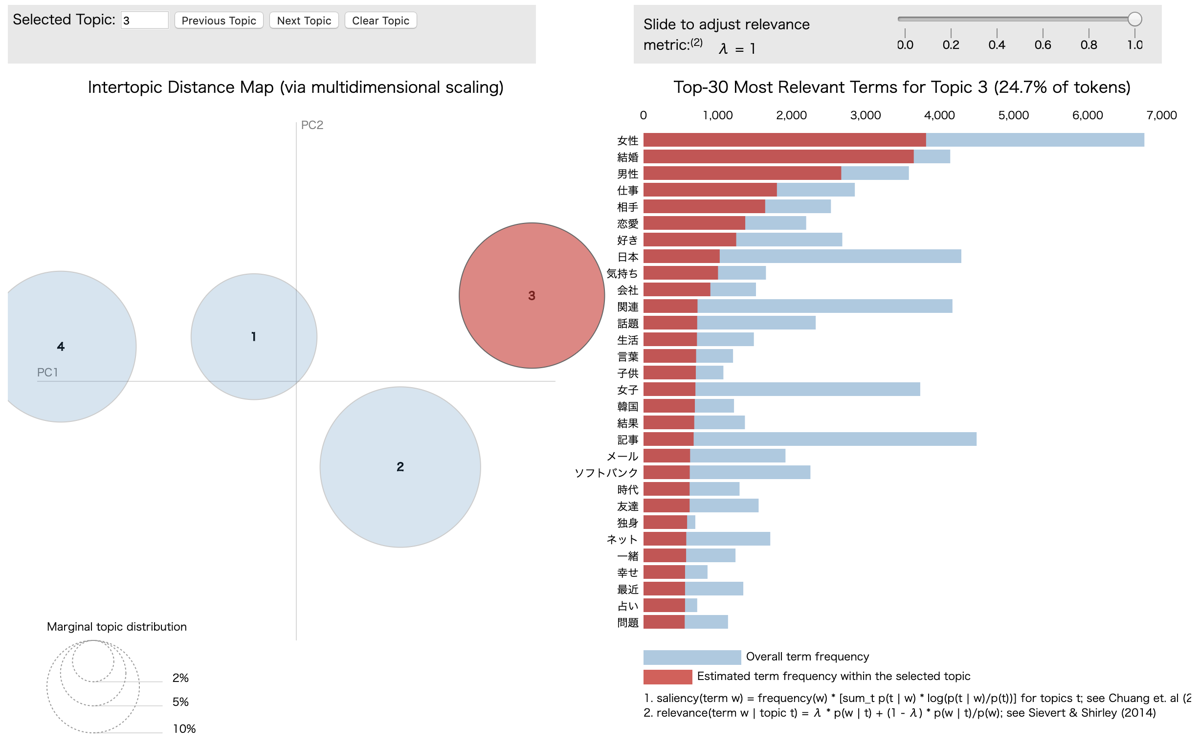
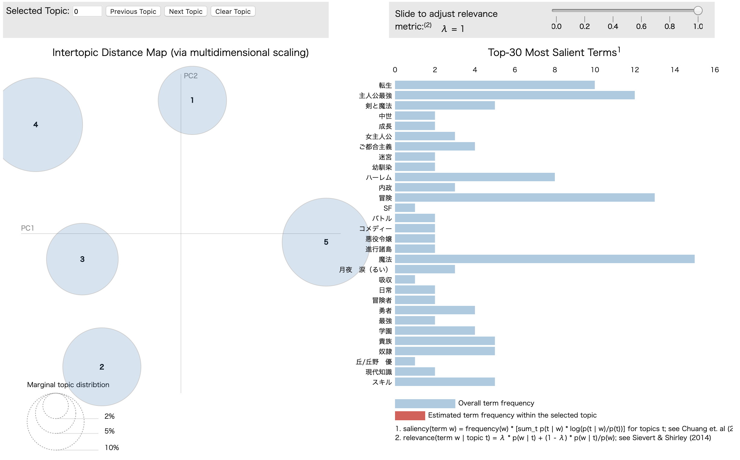
pyLDAvisではインタラクティブに可視化結果を操作できます．
左側の円はそれぞれトピックを，円の大きさはトピックに含まれる文書数を，円と円の距離はトピック間の距離を可視化しています．
右側は単語の発生頻度を表しており，トピックを選択するとそのトピック内での単語の発生頻度を見ることができます．
この可視化結果から，分布の近い，または重なるトピックが複数存在することが分かるため，トピック数を減らしてみます．

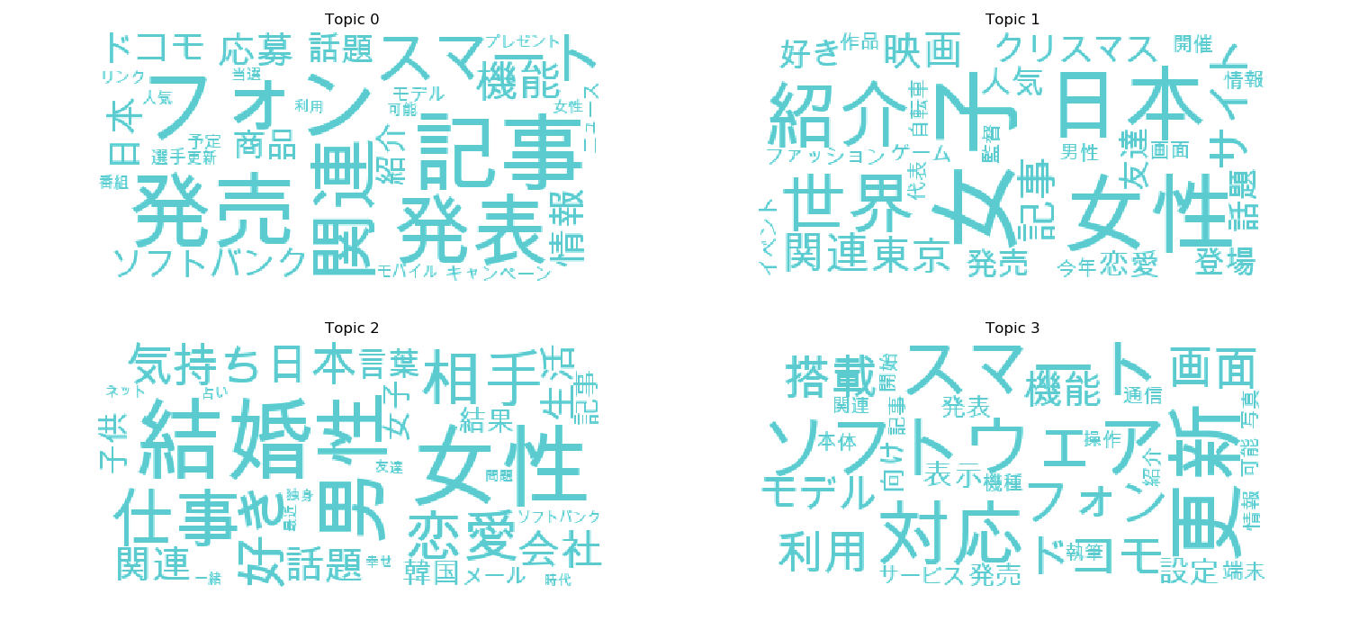
以下はトピック数を4にした場合の可視化結果です．
トピック数が10の場合と比べてトピックの分布がバラけたことが分かります（トピック数が適切であるかどうかは別として）．
WordCloudによる可視化結果から，

Topic 0, 3は携帯電話関連
Topic 1は女性の趣味関連
Topic 2は恋愛関連

のトピックであるように思えなくもないです．

これらを通して適切なトピック数の選択や得られたトピックの解釈，評価が難しいことが分かります．

「小説家になろう」解析

ここでは主にこの記事とこの記事内でやられている内容・コードを拝借しました．
小説を読もう！の累計ランキング上位100をLDAで解析し，作品の傾向を調べます．
ここでは文書ではなく，各作品に付けられている「タグ」を単語とみたててLDAを行います．
こちらについても参考記事内のものとほぼ同じですが，ソースコードを以下に示します．

ソースコード

必要ライブラリのインポート等

import urllib.request, urllib.error
from bs4 import BeautifulSoup
import gensim
import matplotlib.pylab as plt
from wordcloud import WordCloud

FONT = "/Library/Fonts/Arial Unicode.ttf"

サイトから各作品のタグを取得する関数を定義

def getNarouRankingHTML():
    return urllib.request.urlopen('http://yomou.syosetu.com/rank/list/type/total_total/')

def getNarouRankingTags(soup):
    return [[item.string for item in div.find_all('a') if item.string != None] for div in soup.find_all(class_='ranking_list')]

トピックの分布間のKL divergence を計算する関数を定義

def calc_topic_distances(m, topic):
    import numpy as np

    def kldiv(p, q):
        distance = np.sum(p * np.log(p / q))
        return distance

    # get probability of each words
    # https://github.com/piskvorky/gensim/blob/develop/gensim/models/ldamodel.py#L733

    t = m.state.get_lambda()
    for i, p in enumerate(t):
        t[i] = t[i] / t[i].sum()

    base = t[topic]
    distances = [(i_p[0], kldiv(base, i_p[1])) for i_p in enumerate(t) if i_p[0] != topic]
    return distances

def plot_distance_matrix(m):
    import numpy as np
    import matplotlib.pylab as plt

    # make distance matrix
    mt = []
    for i in range(m.num_topics):
        d = calc_topic_distances(m, i)
        d.insert(i, (i, 0))  # distance between same topic
        d = [_d[1] for _d in d]
        mt.append(d)

    mt = np.array(mt)

    # plot matrix
    fig = plt.figure()
    ax = fig.add_subplot(1, 1, 1)
    ax.set_aspect("equal")
    plt.imshow(mt, interpolation="nearest", cmap=plt.cm.ocean)
    plt.yticks(range(mt.shape[0]))
    plt.xticks(range(mt.shape[1]))
    plt.colorbar()
    plt.savefig("./kldiv.png")

辞書とコーパスの作成からLDAの実行
5割以上の文書に登場する単語をフィルタリングし，トピック数を10に設定しています．

soup = BeautifulSoup(html, "lxml")
tags = getNarouRankingTags(soup)[:100]  # best 100

print("num tags : ", len(tags))
dictionary = gensim.corpora.Dictionary(tags)
dictionary.filter_extremes(no_below=1, no_above=0.5)
print("len dictionary : ", len(dictionary))

corpus = [dictionary.doc2bow(tag) for tag in tags]

# LDA
num_topics = 10
lda = gensim.models.ldamodel.LdaModel(corpus=corpus, num_topics=num_topics, id2word=dictionary, random_state=0)
# output tags in topics
for x in lda.show_topics(-1, 5):
    print(x)

KL divergence, WordCloud, pyLDAvisによる可視化

# KL divergence
plot_distance_matrix(lda)

# WordCloud
plt.figure(figsize=(30, 30))
for t in range(lda.num_topics):
    plt.subplot(5, 4, t+1)
    x = dict(lda.show_topic(t, 200))
    im = WordCloud(font_path=FONT).generate_from_frequencies(x)
    plt.imshow(im)
    plt.axis("off")
    plt.title("Topic #" + str(t))
plt.savefig("./visualize.png")

# pyLDAvis
vis = pyLDAvis.gensim.prepare(lda, corpus, dictionary, sort_topics=False)
pyLDAvis.save_html(vis, './pyldavis_output.html')

結果

以下が実行結果です．各トピックにおける単語の発生頻度を出力しています．
「異世界〜」が頻出していることが分かります．

num tags :  100
len dictionary :  632
(0, '0.027*"異世界転生" + 0.025*"ファンタジー" + 0.024*"主人公最強" + 0.022*"異世界" + 0.018*"書籍化"')
(1, '0.030*"異世界" + 0.019*"異世界転移" + 0.018*"チート" + 0.018*"ハーレム" + 0.015*"主人公最強"')
(2, '0.022*"異世界" + 0.022*"チート" + 0.015*"異世界転移" + 0.015*"ファンタジー" + 0.015*"魔法"')
(3, '0.030*"異世界" + 0.029*"冒険" + 0.026*"ファンタジー" + 0.021*"魔法" + 0.015*"勇者"')
(4, '0.055*"異世界転移" + 0.036*"異世界" + 0.033*"ファンタジー" + 0.021*"チート" + 0.019*"冒険"')
(5, '0.050*"異世界転生" + 0.040*"異世界" + 0.019*"主人公最強" + 0.017*"転生" + 0.016*"魔法"')
(6, '0.038*"異世界転生" + 0.022*"異世界転移" + 0.018*"冒険" + 0.018*"魔法" + 0.017*"ファンタジー"')
(7, '0.036*"異世界転移" + 0.033*"異世界" + 0.018*"異世界転生" + 0.017*"男主人公" + 0.017*"冒険"')
(8, '0.011*"異世界" + 0.011*"異世界転移" + 0.011*"ファンタジー" + 0.011*"魔法" + 0.011*"成り上がり"')
(9, '0.029*"チート" + 0.023*"異世界転移" + 0.023*"スキル" + 0.021*"異世界転生" + 0.018*"主人公最強"')

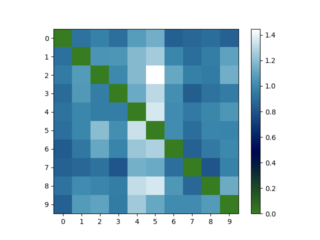
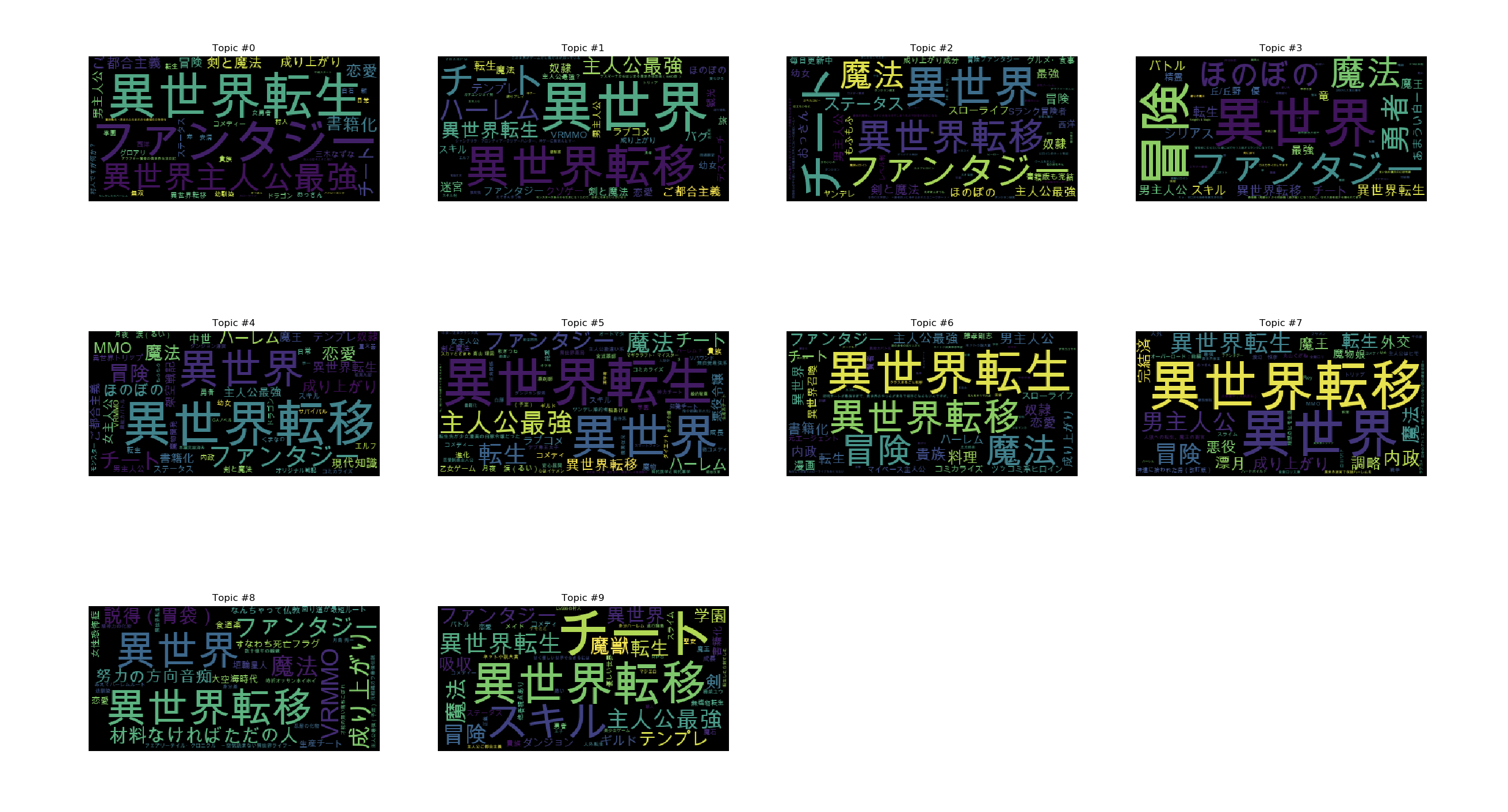
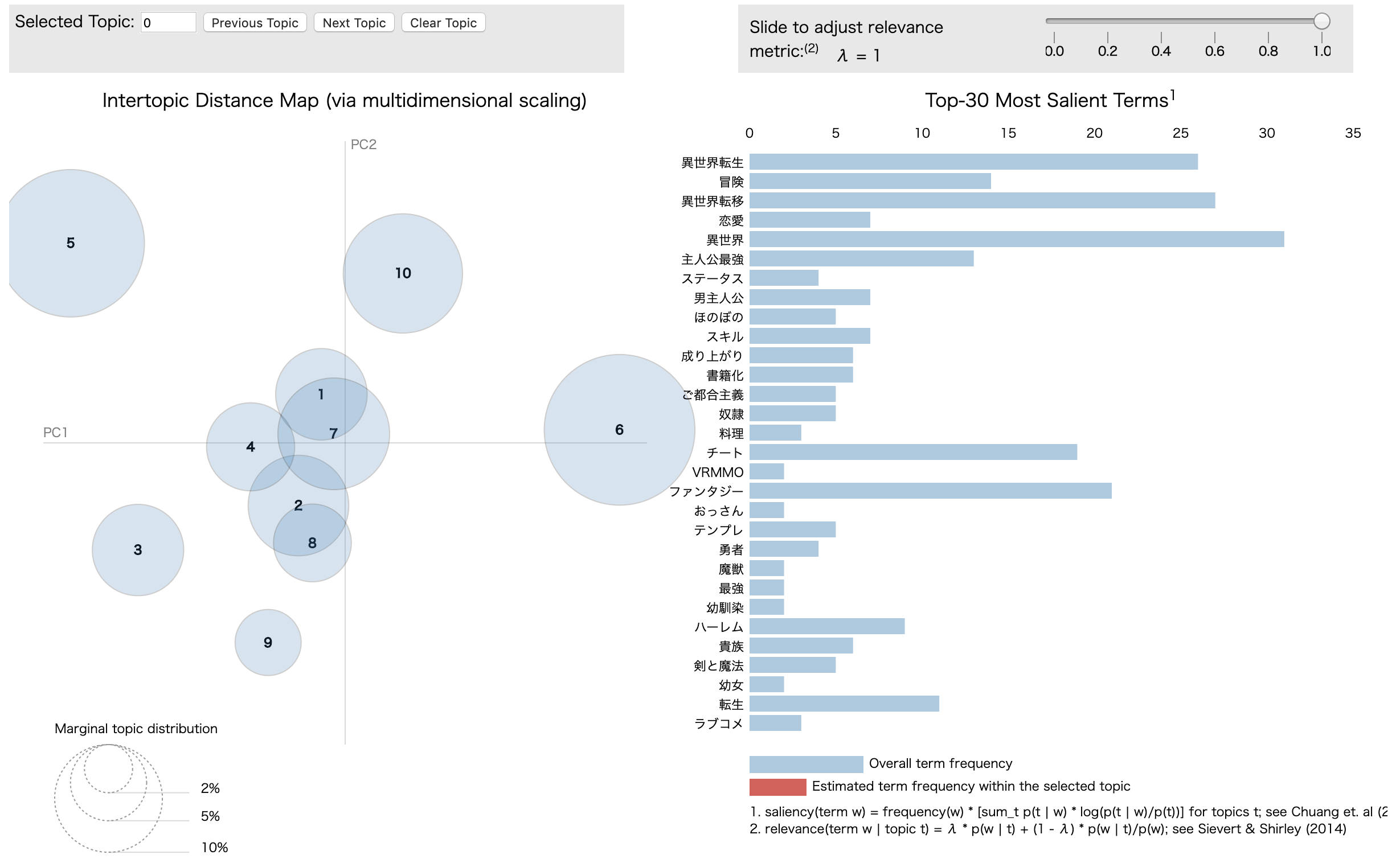
以下はKL divergence, WordCloud, pyLDAvisによる可視化結果です．
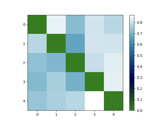
KL divergenceの可視化ではトピックの分布間の距離を行列で表しています．異なるトピック間の距離が大きいほど，つまり対角成分以外が大きな値を持っているほど良いモデルであると言えます．多くの要素が大きな値を持っているので，トピック数を減らしても良いかもしれません．

WordCloudとpyLDAvisによる可視化結果からやはりどのトピックでも「異世界〜」が登場し，また複数のトピックの分布が重なっていることが分かります．

以上を踏まえて今回は，

2.5割以上の文書に登場する単語（異世界〜）をフィルタリング
トピック数を5

に変更してみます．この場合の結果は以下のようになります．

num tags :  100
len dictionary :  627
(0, '0.019*"転生" + 0.018*"冒険" + 0.012*"ご都合主義" + 0.008*"男主人公" + 0.008*"魔法"')
(1, '0.026*"魔法" + 0.019*"冒険" + 0.011*"恋愛" + 0.009*"主人公最強" + 0.008*"書籍化"')
(2, '0.012*"中世" + 0.012*"ハーレム" + 0.011*"ほのぼの" + 0.010*"魔法" + 0.009*"スキル"')
(3, '0.020*"魔法" + 0.018*"転生" + 0.017*"冒険" + 0.011*"女主人公" + 0.010*"貴族"')
(4, '0.031*"主人公最強" + 0.018*"ハーレム" + 0.015*"剣と魔法" + 0.013*"魔法" + 0.009*"魔王"')

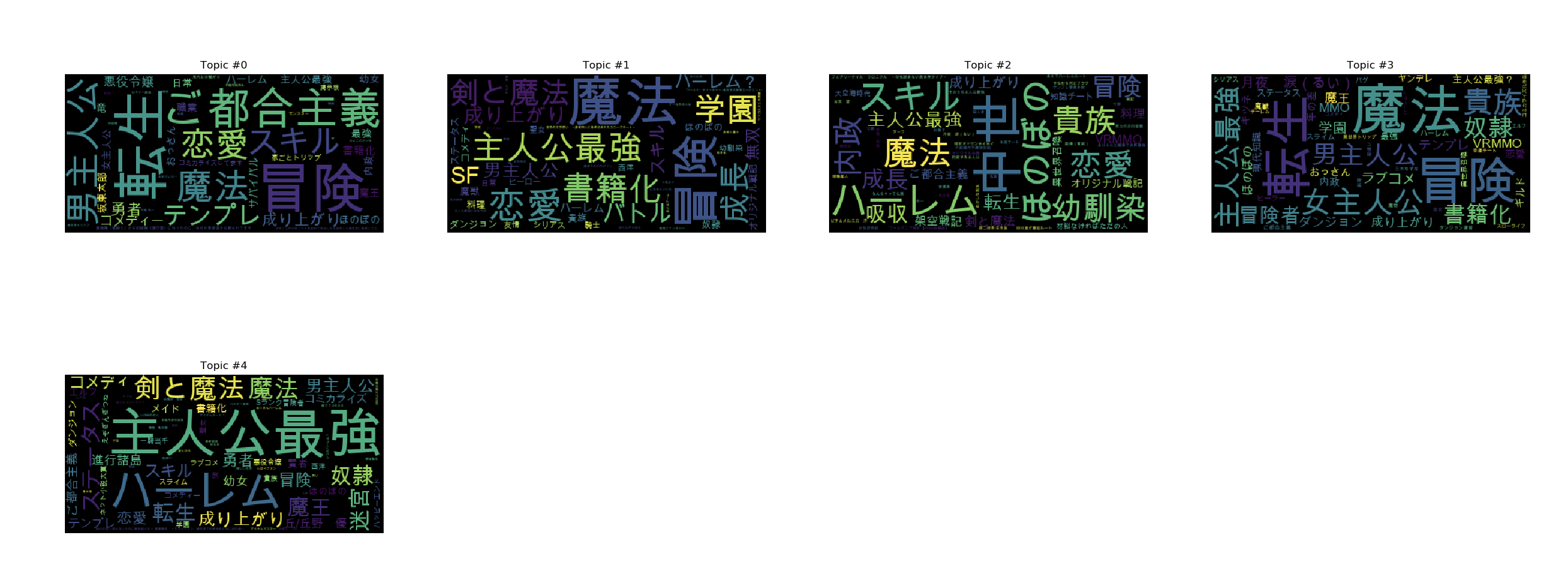
変更前と比較して，

KL divergence の可視化から，どのトピック間の距離もほぼ均等に
WordCloudとpyLDAvisによる可視化から，各トピックが持つ属性が分かりやすく

なりました．

まとめ

ネット上の様々な記事を通してザックリとトピックモデルを理解し，Pythonで試してみました．
教師なし学習ということでトピックの解釈や難しかったり，ハイパーパラメータの調整が非常に重要であることが分かりました．

トピックモデルをザックリと理解してサクッと試した

はじめに

実行環境

参考記事・文献

トピックモデルとは

ニュース記事解析

ソースコード

結果

「小説家になろう」解析

ソースコード

結果

まとめ