機械学習でよく言われる、「隠れ層一層のニューラルネットワークは任意の関数を近似できる」ということを実際に確かめてみよう。隠れ層を一層として、ユニット数を増やしてみる。
TensorFlowを用いる。
基本的なことは
TensorFlowの高レベルAPIの使用方法2:Dataset APIを使ってみる
https://qiita.com/cometscome_phys/items/a95a91f9822353303dd8
を参照のこと。
バージョン
TensorFlow: 1.9.0
Python: 3.6.4
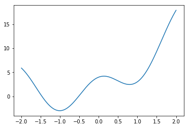
再現すべき関数
ここでは、ある関数
$$
y = a_0 x+ a_1 x^2 + b_0 + 3cos(\alpha x)
$$
という関数を考える。これまでは、最後のcosはノイズのようなものとして考えており、$a_0$と$a_1$と$b_0$によって得られる二次関数を得ることが目的としていた。今回は、この関数自体をフィッティングすることを目指す。$\alpha$を大きくすると振動が増え、より一致が難しくなる。
$\alpha = 3$としてみよう。
データを300点作っておく。
import tensorflow as tf
import numpy as np
import matplotlib.pyplot as plt
%matplotlib inline

n = 300
x0 = np.linspace(-2.0, 2.0, n)
a0 = 3.0
a1 = 2.0
b0 = 1.0
kk = 3
y0 = np.zeros(n)
y0[:] = a0*x0+a1*x0**2 + b0 + 3*np.cos(kk*x0)

plt.plot(x0,y0 )
plt.show()
plt.savefig("graph.png")
この時のグラフは以下の通りである。
これまではデータのフィッティングには多項式による展開をしていたが、今回は、$x$座標そのものを用いる。
つまり、インプットデータは$x$座標、教師データは$y$座標である。
インプットデータの生成
ここはこれまでの記事とほとんど同じである。
$x$そのものをインプットデータとするので、
def make_phi(x0,n,k):
    phi = np.array([x0])
#    phi = np.array([x0**j for j in range(k)])
    return phi.T
という形でインプットデータを生成することにする。ここで$n$はデータの数である。前回のコードを使いまわしているので$k$があるが、この記事では使わない。
データの範囲は-2から2とすると
x0 = np.linspace(-2.0, 2.0, n)
k = 1
phi = make_phi(x0,n,k)
となる。
その時の教師データはy0である。
また、学習には使わない「テストデータ」を100点用意し、
n_test = 100
x0_test = np.linspace(-2.0, 2.0, n_test)
y0_test = np.zeros(n_test)
y0_test[:] = a0*x0_test+a1*x0_test**2 + b0 + 3*np.cos(kk*x0_test)
phi_test = make_phi(x0_test,n_test,k)
としておく。
Dataset APIの使用
ここは前回の記事と同じなので、コードだけ再掲する。
今、バッチサイズを20としている。
batch_size = 20
dataset = tf.data.Dataset.from_tensor_slices({"phi":phi, "y0":y0}).shuffle(10).batch(batch_size)

test_dataset = tf.data.Dataset.from_tensor_slices({"phi":phi_test, "y0":y0_test}).batch(n_test)
iterator = tf.data.Iterator.from_structure(dataset.output_types,
                                           dataset.output_shapes)
train_init_op = iterator.make_initializer(dataset)
test_init_op = iterator.make_initializer(test_dataset)
next_step= iterator.get_next()
となる。
グラフの構築
グラフの構築も前回の記事と同様。
def build_graph_layers_class(d_input,d_middle,d_type):
    x = next_step["phi"]
    yout= next_step["y0"]
    hidden1 = tf.layers.Dense(units=d_middle,activation=tf.nn.relu)
    x1 = hidden1(x)
    outlayer = tf.layers.Dense(units=1,activation=None)
    y = outlayer(x1)

    diff = tf.subtract(y,yout)
    loss = tf.nn.l2_loss(diff)
    minimize = tf.train.AdamOptimizer().minimize(loss)
    return x,y,yout,diff,loss,minimize,hidden1,outlayer
隠れ層1層としてそのユニットを10であるとして、グラフを作る。
d_type = tf.float32
d_input = 1
d_middle = 10
x,y,yout,diff,loss,minimize,hidden1,outlayer= build_graph_layers_class(d_input,d_middle,d_type)
で設定する。d_middleが隠れ層のユニットの数である。
学習
学習についても前回と同じであり、
np = 5000
with tf.Session() as sess:
    tf.global_variables_initializer().run()
    for i in range(np):
        sess.run(train_init_op)
        while True:
            try:
                sess.run(minimize)
                #print(sess.run(next_step))
                losstrain = sess.run(loss)/batch_size
                #print(losstrain)


            except tf.errors.OutOfRangeError:
                break

        sess.run(test_init_op)
        losstest = sess.run(loss)/n_test
        if i % 100 is 0:
            print("i",i,"loss",losstest)
    W = sess.run(hidden1.weights)
    print(W)
    a = sess.run(outlayer.weights)
    print(a)
    sess.run(test_init_op)
    yt = sess.run(y)

plt.plot(x0_test,y0_test )
plt.plot(x0_test,yt )
plt.show()
plt.savefig("graph2.png")
となる。
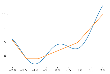
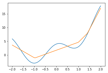
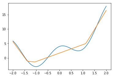
結果
それでは、ユニット数を変化させたときにどうなるか見てみよう。学習はどれも5000回で止めている。
d_type = tf.float32
d_input = 1
d_middle = 10
x,y,yout,diff,loss,minimize,hidden1,outlayer= build_graph_layers_class(d_input,d_middle,d_type)
のd_middleを変えて再実行すればよい。
まず、$\alpha = 3$とする。
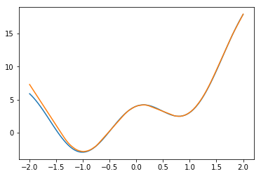
ユニット数4
ユニット数10
ユニット数20
ユニット数50
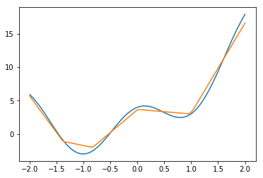
ユニット数100
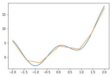
ユニット数200
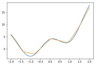
ユニット数500
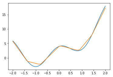
だんだん良くなっている気はするが、思ったよりも上がっていないような気もする。
ユニット数500。データ数3000
Dataset APIに入れたデータは300個だったが、これを10倍すると何か変わるだろうか?
とても綺麗になった。
ユニット数50。データ数3000
データ数は多いままユニット数を1/10にしてみた。

あれ、ユニット数500とあまり変わらなく、良い感じ。
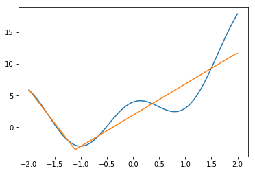
ユニット数10。データ数3000
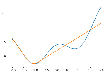
さすがにこれは少なかったらしい。
結論
データ数重要。
(18/08/03)追記
activation関数を変化させたときにどうなるのか、というコメントがあったので、試しに変えてみた。
先ほどまで使っていたactivation関数はReLUと呼ばれるもので、
$$
f(x) = max(0,x)
$$
というものであった。これは、xが0より小さいときには0を、xが0より大きいときはxそのものを返す関数である。
activation関数には他にもあり、例えばシグモイド(sigmoid)関数は
$$
f(x) = \frac{1}{1+\exp(-x)}
$$
である。$x$が0より小さいときはほとんどゼロで、$x=0$の時には1/2、$x$が大きくなっていくと1になる関数である。
TensorFlowでは、activation=tf.nn.reluの代わりにactivation=tf.sigmoidを使えば、シグモイド関数に変更できる。
activation関数の影響がわかりやすいように、ユニット数を2とする。
d_type = tf.float32
d_input = 1
d_middle = 2
x,y,yout,diff,loss,minimize,hidden1,outlayer= build_graph_layers_class(d_input,d_middle,d_type)
データ点は3000点としておく。
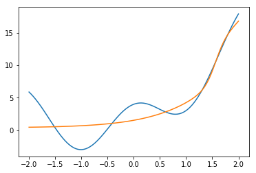
ReLUの場合
これは先ほどと同じactivation関数である。
結果は、
である。今、隠れ層が1層なので、ユニット数が2個ということは二つの原点の異なるReLU関数の重ね合わせということである。
実際、カクカクっとしていて、そうなっていることがわかる。
シグモイドの場合
シグモイドの場合には、
グラフを
def build_graph_layers_class(d_input,d_middle,d_type):
    x = next_step["phi"]
    yout= next_step["y0"]
    hidden1 = tf.layers.Dense(units=d_middle,activation=tf.sigmoid)
    x1 = hidden1(x)
    outlayer = tf.layers.Dense(units=1,activation=None)
    y = outlayer(x1)

    diff = tf.subtract(y,yout)
    loss = tf.nn.l2_loss(diff)
    minimize = tf.train.AdamOptimizer().minimize(loss)
    return x,y,yout,diff,loss,minimize,hidden1,outlayer
と一箇所変更して、
d_type = tf.float32
d_input = 1
d_middle = 2
x,y,yout,diff,loss,minimize,hidden1,outlayer= build_graph_layers_class(d_input,d_middle,d_type)
を再実行する。その結果、
となる。
sigmoid関数はゆっくり変化する関数なので、こちらのがふんわりしている。