はじめに
以前「衛星データでつくばみらい市の変化を見てみた(地理空間データ解析)」という記事を書いた。
衛星データによるバンド演算結果可視化やクラスタリング、モラン$I$統計量の計算などをPythonで実施するという内容だった。
ただあまり、空間統計には踏み込まなかったので、今回は条件付き自己回帰モデル(Conditional Auto-Regressive model;CAR model)で空間データのモデリングを実施していく。
やることを分けると以下の順で6つある。
- 衛星データダウンロード
- 小地域の境界データダウンロード
- 衛星データの前処理
- 土壌分類データダウンロード
- バンド演算
- モデル構築(多項分類)
1~3は「衛星データでつくばみらい市の変化を見てみた(地理空間データ解析)」で実施済みなので、今回は省略する。(コードだけ載せておく。)
土壌分類の学習データは国土数値情報ダウンロードサイト 土地利用細分メッシュデータを利用する。
バンド演算は前回はNDVI、NDBI、BAの3種しかしていなかったが、今回は11種演算し、モデリングの際の説明変数とする。
モデリングでは、多項ロジスティック回帰モデル、ベイズ多項ロジスティック回帰モデル、多項ICARモデル、LightGBMによるモデル構築と検証を行う。
参考
前回も参考にしたもの
- [書籍]Pythonで学ぶ衛星データ解析基礎 環境変化を定量的に把握しよう
- [書籍]Rではじめる地理空間データの統計解析入門
- [Github]Pythonで学ぶ衛星データ解析基礎 環境変化を定量的に把握しよう
- Rasterio公式
- GeoPandas公式
- rasterstats公式
- EarthPy公式
- Shapely公式
- PySAL公式
- libpysal公式
- Raster Resampling for Discrete and Continuous Data
- Copernicus Browser(Sentinel衛星のデータをダウンロードできる)
- GISデータ一覧 行政区域データ
- 境界データ(市町村):国土数値情報ダウンロードサイト
- 境界データ(小地域(町丁・字等別)):e-Stat
- EPSGコード一覧表/日本でよく利用される空間座標系(座標参照系)
- 課題に応じて変幻自在? 衛星データをブレンドして見えるモノ・コト #マンガでわかる衛星データ
- 衛星スペクトル指標を用いた都市化の画像解析
- 森林分野における衛星データ利用事例
- 漁業での衛星データ利用事例
- Sentinel-2 Imagery: NDVI Raw
- Sentinel-2 Imagery: Normalized Difference Built-Up Index (NDBI)
- esrij ジャパン GIS 基礎解説 リサンプリング
- つくばみらい市のホームページ
今回から参考にしたもの
- 国土数値情報ダウンロードサイト 土地利用細分メッシュデータ
- ICARモデルのMCMCをPythonで実行する
- NumPyro:再パラメータ化
- 実験!岩波データサイエンス1のベイズモデリングをPyMC Ver.5で⑨空間自己回帰モデル:1次元の個体数カウントデータ
- 実験!岩波データサイエンス1のベイズモデリングをPyMC Ver.5で⑩空間自己回帰モデル:2次元の株数カウントデータ
- Bayesian Analysis with PyMC 勉強ノート 5 分類モデル
- 衛星データでつくばみらい市の変化を見てみた(地理空間データ解析)
- 階層ベイズで個性を捉える(PyMC ver.5.7.2)
- [書籍]RとStanではじめる ベイズ統計モデリングによるデータ分析入門
- PyMC公式
- [PyMC Discourse Forum]How to perform weighted inference
- [PyMC Discourse Forum]How to run logistic regression with weighted samples
- [PyMC Discourse Forum]Pm.sample_posterior_predictive() not working with weights
- [PyMC Discourse Forum]UserWarning: The effect of Potentials on other parameters is ignored during prior predictive sampling. This is likely to lead to invalid or biased predictive samples
- [PDF file]条件付自己回帰モデルによる空間自己相関を考慮した生物の分布データ解析
- [書籍]基礎からわかるリモートセンシング
- Sentinel-2A / 2B / 2C / 2D 概要
- esri 指数ギャラリー
- Index Formula List
- [PDF file]時系列LANDSATデータによる足尾荒廃山地における植生回復モニタリング
- (研究成果) 水田の代かき時期を衛星データで広域把握 用語の解説:MNDWI
- [PDF file]尾瀬地域における衛星リモートセンシングによる植生モニタリング手法の検討
- [PDF file]植物群落内放射伝達モデルを用いたマルチスペクトルカメラの違いによる水田観測結果への影響評価
- [PDF file]Impervious Surface Extraction by Linear Spectral Mixture Analysis with Post-Processing Model
- [PDF file]Developing soil indices based on brightness, darkness, and greenness to improve land surface mapping accuracy
環境
使用環境はGoogle Colaboratory。
以下のパッケージをpipでインストールする。(使っていないやつもあるけど…。)
!pip install geopandas
!pip install earthpy
!pip install rasterio
!pip install sentinelsat
!pip install cartopy
!pip install fiona
!pip install shapely
!pip install pyproj
!pip install pygeos
!pip install rtree
!pip install rioxarray
!pip install pystac-client sat-search
!pip install rich
!pip install rasterstats
!pip install pysal
!pip install libpysal
!pip install geoplot
!pip install optuna
!pip install optuna-integration
!pip install japanize-matplotlib
Google Driveをマウントしておく。
from google.colab import drive
drive.mount('/content/drive')
使用パッケージimport
#必要ライブラリのインポート
import numpy as np
from scipy.ndimage import gaussian_filter
from scipy.special import softmax
import pandas as pd
import matplotlib
import matplotlib.pyplot as plt
import matplotlib.image as mpimg
import matplotlib.ticker as ptick
import matplotlib.font_manager as fm
from matplotlib.colors import BoundaryNorm
from matplotlib.cm import get_cmap
import japanize_matplotlib

import seaborn as sns
import mpl_toolkits
from mpl_toolkits.axes_grid1 import make_axes_locatable
import sklearn
import sklearn.cluster
import sklearn.metrics
from sklearn import preprocessing
import rich.table
import xarray as xr
import rioxarray as rxr

import geopandas as gpd
import geoplot as gplt
import cartopy, fiona, shapely, pyproj, rtree, pygeos
import cv2
import rasterio as rio
from rasterio import plot
from rasterio.plot import show, plotting_extent
from rasterio.mask import mask
from rasterio.enums import Resampling
from rasterio.features import geometry_mask, shapes
from shapely.geometry import MultiPolygon, Polygon, shape
import rasterstats
import earthpy.spatial as es
import earthpy.plot as ep
import libpysal

import os
import zipfile
import glob
import shutil

import urllib
from satsearch import Search
from pystac_client import Client
from PIL import Image
import requests
import io
from pystac_client import Client
import warnings
# from tqdm import tqdm
from tqdm.notebook import tqdm

import pymc as pm
import jax
import arviz as az
import pytensor.tensor as pt
import pytensor
import gc
import optuna.integration.lightgbm as opt_lgb

# CPU Multi
os.environ["XLA_FLAGS"] = '--xla_force_host_platform_device_count=8'
print(jax.default_backend())
print(jax.devices("cpu"))

# 日本語フォント読み込み
japanize_matplotlib.japanize()
# jpn_fonts=list(np.sort([ttf for ttf in fm.findSystemFonts() if 'ipaexg' in ttf or 'msgothic' in ttf or 'japan' in ttf or 'ipafont' in ttf]))
# jpn_font=jpn_fonts[0]
jpn_font = japanize_matplotlib.get_font_ttf_path()
prop = fm.FontProperties(fname=jpn_font)
print(jpn_font)
plt.rcParams['font.family'] = prop.get_name() #全体のフォントを設定
plt.rcParams['figure.dpi'] = 250

pd.options.display.float_format = '{:.5f}'.format
sns.set()
衛星データ・小地域の境界データダウンロード(説明省略)
使用するバンドは、'B12','B11','B08','B04','B03','B02'(SWIR2, SWIR1, NIR, RED, GREEN, BLUE)の6種。
ダウンロード方法の詳細は「[書籍]Pythonで学ぶ衛星データ解析基礎 環境変化を定量的に把握しよう」か、「衛星データでつくばみらい市の変化を見てみた(地理空間データ解析)」を参照。
小地域境界データもe-Statからダウンロードしておく。(e-Stat)
衛星データのダウンロードコード(折り畳み)
# データをダウンロードするかどうか
DOWNLOAD = False

# 保存するディレクトリの作成
dst_dir = '/content/drive/MyDrive/satelite/s2Bands'  # Google Colabでは'/content~~'が正
os.makedirs(dst_dir, exist_ok=True)

# 座標の基準とするラスターデータ読み込み
raster_crs = rio.open(os.path.join(dst_dir,'S2B_54SVE_20180428_0_L2A_B11.tif'))
raster_profile = raster_crs.profile

# 小地域区分のベクターデータ(from e-Stat)を読み込みcrsをラスターデータに合わせる
shape_path = "/content/drive/MyDrive/satelite/ibrakiPolygon/"  # Google Colabでは'/content~~'が正
os.makedirs(shape_path, exist_ok=True)
part_in_shape = gpd.read_file(os.path.join(shape_path, "r2ka08235.shp"), encoding="shift-jis")[['PREF_NAME', 'CITY_NAME', 'S_NAME', 'AREA', 'PERIMETER', 'JINKO', 'SETAI', 'geometry']]
re_shape_tsukuba_mirai_2RasterCrs = part_in_shape.to_crs(raster_profile["crs"])  #crs合わせ
print(re_shape_tsukuba_mirai_2RasterCrs.shape)
# 同じ小地域がさらに細かく分かれている場合があるので、小地域単位でグループ化しておく
re_shape_tsukuba_mirai_2RasterCrs = re_shape_tsukuba_mirai_2RasterCrs.dissolve(['PREF_NAME', 'CITY_NAME', 'S_NAME'], aggfunc='sum', as_index=False)
print(re_shape_tsukuba_mirai_2RasterCrs.shape)  # 特定の小地域が統合されレコード数が減る
display(re_shape_tsukuba_mirai_2RasterCrs)


# 取得範囲を指定するための関数を定義
def selSquare(lon, lat, delta_lon, delta_lat):
    c1 = [lon + delta_lon, lat + delta_lat]
    c2 = [lon + delta_lon, lat - delta_lat]
    c3 = [lon - delta_lon, lat - delta_lat]
    c4 = [lon - delta_lon, lat + delta_lat]
    geometry = {"type": "Polygon", "coordinates": [[ c1, c2, c3, c4, c1 ]]}
    return geometry

# 茨城県周辺の緯度経度をbbox内へ
geometry = selSquare(140.0363, 35.9632, 0.06, 0.02)
timeRange = '2018-01-01/2023-12-31' # 取得時間範囲を指定

# STACサーバに接続し、取得範囲・時期やクエリを与えて取得するデータを絞る
# sentinel:valid_cloud_coverを用いて、雲量の予測をより確からしいもののみに限定している
if DOWNLOAD:
  api_url = 'https://earth-search.aws.element84.com/v0'
  collection = "sentinel-s2-l2a-cogs"  # Sentinel-2, Level 2A (BOA)
  s2STAC = Client.open(api_url, headers=[])
  s2STAC.add_conforms_to("ITEM_SEARCH")

  s2Search = s2STAC.search (
      intersects = geometry,
      datetime = timeRange,
      query = {"eo:cloud_cover": {"lt": 11}, "sentinel:valid_cloud_cover": {"eq": True}},
      collections = collection)

  s2_items = [i.to_dict() for i in s2Search.get_items()]
  print(f"{len(s2_items)} のシーンを取得")

# product_idやそのgeometryの情報がまとまったdf作成
if DOWNLOAD:
  items = s2Search.get_all_items()
  df = gpd.GeoDataFrame.from_features(items.to_dict(), crs="epsg:32654")
  dfSorted = df.sort_values('eo:cloud_cover').reset_index(drop=True)
  # epsgの種類
  print('epsg', dfSorted['proj:epsg'].unique())
  display(dfSorted.head(3))
  # 雲量10以下の日時
  print(np.sort(dfSorted[dfSorted['eo:cloud_cover']<=10]['datetime'].unique()))

# 2018‐2023各年の同じ時期のproduct_id一覧取得
if DOWNLOAD:
  df_selected = dfSorted[dfSorted['datetime'].isin(['2018-04-28T01:36:01Z', '2019-05-08T01:37:21Z', '2020-05-02T01:37:21Z', '2021-04-22T01:37:12Z', '2022-04-12T01:37:20Z', '2023-04-27T01:37:18Z'])].copy().sort_values('datetime').iloc[[0,2,3,4,5,6],:]
  display(df_selected['sentinel:product_id'].to_list())

# 各productのデータURLやtifファイル名の一覧取得
if DOWNLOAD:
  selected_item = [x.assets for x in items if x.properties['sentinel:product_id'] in (df_selected['sentinel:product_id'].to_list())]
  selected_item = sorted(selected_item, key=lambda x:x['thumbnail'].href)

# thumbnailで撮影領域確認
if DOWNLOAD:
  plt.rcParams['font.family'] = prop.get_name() #全体のフォントを設定
  fig = plt.figure(figsize=(7,3))
  for ix, sitm in enumerate(selected_item):
    thumbImg = Image.open(io.BytesIO(requests.get(sitm['thumbnail'].href).content))
    ax = plt.subplot(2,3,ix+1)
    ax.imshow(thumbImg)
    plt.setp(ax.get_xticklabels(), fontsize=4)
    plt.setp(ax.get_yticklabels(), fontsize=4)
    ax.set_title('撮影日時 : '+'-'.join(sitm['thumbnail'].href.split('/')[-5:-2]), fontsize=4)
    ax.grid(False)
  plt.tight_layout()
  plt.show()

# Sentinel-2のバンド情報を表で示す
if DOWNLOAD:
  table = rich.table.Table("Asset Key", "Description")
  for asset_key, asset in selected_item[0].items():
    table.add_row(asset_key, asset.title)

  display(table)

# URLからファイルをダウンロードする関数を定義
# 引用:https://note.nkmk.me/python-download-web-images/
def download_file(url, dst_path):
    try:
        with urllib.request.urlopen(url) as web_file, open(dst_path, 'wb') as local_file:
            local_file.write(web_file.read())
    except urllib.error.URLError as e:
        print(e)

def download_file_to_dir(url, dst_dir):
    download_file(url, os.path.join(dst_dir, url.split('/')[-2]+'_'+os.path.basename(url)))


# tifファイルをダウンロード(時間かかる)
if DOWNLOAD:
  # 取得するバンドの選択
  bandLists = ['B12','B11','B08','B04','B03','B02'] # SWIR2, SWIR1, NIR, RED, GREEN, BLUE

  # 画像のURL取得
  file_url = []
  for sitm in selected_item:
    [file_url.append(sitm[band].href) for band in bandLists if file_url.append(sitm[band].href) is not None]

  # 画像のダウンロード
  [download_file_to_dir(link, dst_dir) for link in file_url if download_file_to_dir(link, dst_dir) is not None]

# ダウンロードファイルリスト(撮影日時順)
display(sorted(os.listdir(dst_dir), key=lambda x:(x.split('_54SVE_')[-1])))

# 試しにバンド11のデータを1つ可視化
src = rio.open(os.path.join(dst_dir,'S2B_54SVE_20180428_0_L2A_B11.tif'))
fig = plt.figure(figsize=(2, 2))
ax=plt.subplot(1,1,1)
retted = show(src.read(), transform=src.transform, cmap='RdYlGn', ax=ax, vmax=np.quantile(src.read(1), q=0.99))
img = retted.get_images()[0]
divider = mpl_toolkits.axes_grid1.make_axes_locatable(ax)
cax = divider.append_axes('right', '5%', pad='3%')
cbar = plt.colorbar(img, cax=cax)
cbar.ax.tick_params(labelsize=4)
plt.setp(ax.get_xticklabels(), fontsize=4)
plt.setp(ax.get_yticklabels(), fontsize=4)
ax.yaxis.offsetText.set_fontsize(4)
ax.yaxis.set_major_formatter(ptick.ScalarFormatter(useMathText=True))
ax.ticklabel_format(style='sci', axis='y', scilimits=(0,0))
ax.grid(False)
plt.show()

# 試しにバンド12のデータを1つ可視化
src = rio.open(os.path.join(dst_dir,'S2B_54SVE_20180428_0_L2A_B12.tif'))
fig = plt.figure(figsize=(2, 2))
ax=plt.subplot(1,1,1)
retted = show(src.read(), transform=src.transform, cmap='RdYlGn', ax=ax, vmax=np.quantile(src.read(1), q=0.99))
img = retted.get_images()[0]
divider = mpl_toolkits.axes_grid1.make_axes_locatable(ax)
cax = divider.append_axes('right', '5%', pad='3%')
cbar = plt.colorbar(img, cax=cax)
cbar.ax.tick_params(labelsize=4)
plt.setp(ax.get_xticklabels(), fontsize=4)
plt.setp(ax.get_yticklabels(), fontsize=4)
ax.yaxis.offsetText.set_fontsize(4)
ax.yaxis.set_major_formatter(ptick.ScalarFormatter(useMathText=True))
ax.ticklabel_format(style='sci', axis='y', scilimits=(0,0))
ax.grid(False)
plt.show()


# ラスターデータリスト読み込み
getList = sorted(list(glob.glob(dst_dir+'/S2*')), key=lambda x:(x.split('_54SVE_')[-1]))
display(getList)

# ラスターデータをベクターデータの範囲にcropして保存
s2Output = '/content/drive/MyDrive/satelite/s2Output'  # Google Colabでは'/content~~'が正
os.makedirs(s2Output, exist_ok=True) # outputデータ保存ディレクトリ
if DOWNLOAD:
  band_paths_list = es.crop_all(list(getList), s2Output, re_shape_tsukuba_mirai_2RasterCrs, overwrite=True)
# cropしたラスターデータリスト
band_paths_list = sorted(list(glob.glob(s2Output+'/S2*')), key=lambda x:(x.split('_54SVE_')[-1]))  # 撮影日時順にソート
display(band_paths_list)

# cropしたラスターデータ(つくばみらい市)をベクターデータと共に試しに可視化
src = rio.open(band_paths_list[3])  # Band 8
fig = plt.figure(figsize=(2, 2))
ax=plt.subplot(1,1,1)
retted = show(src.read(), transform=src.transform, cmap='coolwarm', ax=ax, vmin=0, vmax=3500)
im = retted.get_images()[0]
divider = mpl_toolkits.axes_grid1.make_axes_locatable(ax)
cax = divider.append_axes("right", '5%')
cbar = fig.colorbar(im, ax=ax, cax=cax, shrink=0.6, extend='both')
cbar.ax.tick_params(labelsize=4)
re_shape_tsukuba_mirai_2RasterCrs.plot(facecolor='none', edgecolor='k', alpha=1, ax=ax, linewidth=0.2)
plt.setp(ax.get_xticklabels(), fontsize=4)
plt.setp(ax.get_yticklabels(), fontsize=4)
ax.yaxis.offsetText.set_fontsize(4)
ax.yaxis.set_major_formatter(ptick.ScalarFormatter(useMathText=True))
ax.ticklabel_format(style='sci', axis='y', scilimits=(0,0))
ax.set_title('_'.join(os.path.basename(src.name).split('_')[-5:-1]), fontsize=4)
ax.grid(False)
plt.tight_layout()
plt.show()

# 各バンドのtifファイルのリスト
B04s = sorted(list(glob.glob(os.path.join(s2Output,'S2*B04_crop.tif*'))), key=lambda x:(x.split('_54SVE_')[-1]))
B08s = sorted(list(glob.glob(os.path.join(s2Output,'S2*B08_crop.tif*'))), key=lambda x:(x.split('_54SVE_')[-1]))
B11s = sorted(list(glob.glob(os.path.join(s2Output,'S2*B11_crop.tif*'))), key=lambda x:(x.split('_54SVE_')[-1]))
B12s = sorted(list(glob.glob(os.path.join(s2Output,'S2*B12_crop.tif*'))), key=lambda x:(x.split('_54SVE_')[-1]))

B03s = sorted(list(glob.glob(os.path.join(s2Output,'S2*B03_crop.tif*'))), key=lambda x:(x.split('_54SVE_')[-1]))
B02s = sorted(list(glob.glob(os.path.join(s2Output,'S2*B02_crop.tif*'))), key=lambda x:(x.split('_54SVE_')[-1]))
print(B04s)
print(B08s)
print(B11s)
print(B12s)
print(B03s)
print(B02s)

if DOWNLOAD:
    # バンドごとに分解能が違う場合があるので、リサンプリングしてグリッドを合わせる
    # 10m分解能のバンドを20m分解能のバンド11のグリッドに合わせる
    for num, (b04, b08, b11, b12, b03, b02) in enumerate(zip(B04s, B08s, B11s, B12s, B03s, B02s)):
      print('#####', os.path.basename(b08).split('_')[2], '#####')
      riod04 = rio.open(b04)
      riod08 = rio.open(b08)
      riod11 = rio.open(b11)
      riod12 = rio.open(b12)
      riod03 = rio.open(b03)
      riod02 = rio.open(b02)
      bounds = riod04.bounds
      # print(riod08.read().shape)
      # print(riod11.read().shape)
      # ラスターデータをリサンプリングしてバンド11に合わせる
      riod08_resampling = riod08.read(out_shape=(riod08.count,int(riod11.height),int(riod11.width)),
                                      resampling=Resampling.cubic)
      riod04_resampling = riod04.read(out_shape=(riod04.count,int(riod11.height),int(riod11.width)),
                                      resampling=Resampling.cubic)
      riod03_resampling = riod03.read(out_shape=(riod03.count,int(riod11.height),int(riod11.width)),
                                      resampling=Resampling.cubic)
      riod02_resampling = riod02.read(out_shape=(riod02.count,int(riod11.height),int(riod11.width)),
                                      resampling=Resampling.cubic)

      print('B11', riod11.read().shape, riod11.read().shape, sep='-->')
      print('B12', riod12.read().shape, riod12.read().shape, sep='-->')
      print('B04', riod04.read().shape, riod04_resampling.shape, sep='-->')
      print('B08', riod08.read().shape, riod08_resampling.shape, sep='-->')
      print('B03', riod03.read().shape, riod03_resampling.shape, sep='-->')
      print('B02', riod02.read().shape, riod02_resampling.shape, sep='-->')

      out_meta = riod11.meta
      out_meta.update({'dtype':rio.float32})

      fname11 = 'resampling_'+os.path.basename(riod11.name)
      with rio.open(os.path.join(s2Output, fname11), "w", **out_meta) as dest:
        dest.write(riod11.read().astype(rio.float32))

      fname12 = 'resampling_'+os.path.basename(riod12.name)
      with rio.open(os.path.join(s2Output, fname12), "w", **out_meta) as dest:
        dest.write(riod12.read().astype(rio.float32))

      fname08 = 'resampling_'+os.path.basename(riod08.name)
      with rio.open(os.path.join(s2Output, fname08), "w", **out_meta) as dest:
        dest.write(riod08_resampling.astype(rio.float32))

      fname04 = 'resampling_'+os.path.basename(riod04.name)
      with rio.open(os.path.join(s2Output, fname04), "w", **out_meta) as dest:
        dest.write(riod04_resampling.astype(rio.float32))

      fname03 = 'resampling_'+os.path.basename(riod03.name)
      with rio.open(os.path.join(s2Output, fname03), "w", **out_meta) as dest:
        dest.write(riod03_resampling.astype(rio.float32))

      fname02 = 'resampling_'+os.path.basename(riod02.name)
      with rio.open(os.path.join(s2Output, fname02), "w", **out_meta) as dest:
        dest.write(riod02_resampling.astype(rio.float32))
土壌分類データダウンロード
土壌分類のデータは、国土数値情報ダウンロードサイト 土地利用細分メッシュデータからダウンロードする。
今回は茨城県を含むデータが欲しいので、以下の4メッシュの日本測地系のデータをダウンロードする。

4つのデータをダウンロードしたら、それぞれのデータを小地域境界データを使ってつくばみらい市の範囲に切り取る。
切り取った4つのデータを連結させて、1つのデータにする。
(切り取るための小地域境界ベクターデータ再定義)
# 使用するディレクトリ
dst_dir = '/content/drive/MyDrive/satelite/s2Bands'  # Google Colabでは'/content~~'が正
os.makedirs(dst_dir, exist_ok=True)

shape_path = "/content/drive/MyDrive/satelite/ibrakiPolygon/"  # Google Colabでは'/content~~'が正
os.makedirs(shape_path, exist_ok=True)

s2Output = '/content/drive/MyDrive/satelite/s2Output'  # Google Colabでは'/content~~'が正
os.makedirs(s2Output, exist_ok=True) # outputデータ保存ディレクトリ

# 座標の基準とするラスターデータ読み込み
raster_crs = rio.open(os.path.join(dst_dir,'S2B_54SVE_20180428_0_L2A_B11.tif'))
raster_profile = raster_crs.profile

# 小地域区分のベクターデータ(from e-Stat)を読み込みcrsをラスターデータに合わせる
shape_path = "/content/drive/MyDrive/satelite/ibrakiPolygon/"  # Google Colabでは'/content~~'が正
os.makedirs(shape_path, exist_ok=True)
part_in_shape = gpd.read_file(os.path.join(shape_path, "r2ka08235.shp"), encoding="shift-jis")[['PREF_NAME', 'CITY_NAME', 'S_NAME', 'AREA', 'PERIMETER', 'JINKO', 'SETAI', 'geometry']]
re_shape_tsukuba_mirai_2RasterCrs = part_in_shape.to_crs(raster_profile["crs"])  #crs合わせ
print(re_shape_tsukuba_mirai_2RasterCrs.shape)
# 同じ小地域がさらに細かく分かれている場合があるので、小地域単位でグループ化しておく
re_shape_tsukuba_mirai_2RasterCrs = re_shape_tsukuba_mirai_2RasterCrs.dissolve(['PREF_NAME', 'CITY_NAME', 'S_NAME'], aggfunc='sum', as_index=False)
print(re_shape_tsukuba_mirai_2RasterCrs.shape)  # 特定の小地域が統合されレコード数が減る
display(re_shape_tsukuba_mirai_2RasterCrs)
つくばみらい市の範囲に切り取る。
切り取った4つのデータを連結させて、1つのデータにする。
DOWNLOAD = True
# 茨城県を含む土壌分類のデータをダウンロードしておく(国土数値情報ダウンロードサイト 土地利用細分メッシュデータ4つ)
if DOWNLOAD:
    print(1)
    ground_truth = gpd.read_file(os.path.join(shape_path, "L03-b-21_5340-tky.shp"), encoding="shift-jis")
    ground_truth = ground_truth.to_crs(raster_profile["crs"])  #crs合わせ
    ground_truth = gpd.overlay(re_shape_tsukuba_mirai_2RasterCrs, ground_truth, how='intersection')  # クロップ
    print(2)
    ground_truth2 = gpd.read_file(os.path.join(shape_path, "L03-b-21_5339-tky.shp"), encoding="shift-jis")
    ground_truth2 = ground_truth2.to_crs(raster_profile["crs"])  #crs合わせ
    ground_truth2 = gpd.overlay(re_shape_tsukuba_mirai_2RasterCrs, ground_truth2, how='intersection')
    print(3)
    ground_truth3 = gpd.read_file(os.path.join(shape_path, "L03-b-21_5440-tky.shp"), encoding="shift-jis")
    ground_truth3 = ground_truth3.to_crs(raster_profile["crs"])  #crs合わせ
    ground_truth3 = gpd.overlay(re_shape_tsukuba_mirai_2RasterCrs, ground_truth3, how='intersection')
    print(4)
    ground_truth4 = gpd.read_file(os.path.join(shape_path, "L03-b-21_5439-tky.shp"), encoding="shift-jis")
    ground_truth4 = ground_truth4.to_crs(raster_profile["crs"])  #crs合わせ
    ground_truth4 = gpd.overlay(re_shape_tsukuba_mirai_2RasterCrs, ground_truth4, how='intersection')

# 4つのデータを連結
if DOWNLOAD:
    ground_truth_2RasterCrs_concat = pd.concat([ground_truth
                                                , ground_truth2
                                                , ground_truth3
                                                , ground_truth4]).reset_index(drop=True)
    ground_truth_2RasterCrs_concat.to_file(os.path.join(shape_path, "ground_truth_2RasterCrs_concat.shp"), encoding="shift-jis")

# 連結した土壌分類でデータ読み込み
ground_truth_2RasterCrs_concat = gpd.read_file(os.path.join(shape_path, "ground_truth_2RasterCrs_concat.shp"), encoding="shift-jis")
display(ground_truth_2RasterCrs_concat)

MultiPolygonをPolygonに紐解いて、土壌分類をラベルエンコーディング。
# 一部MultiPolygonの地域があるのでPolygonに紐解いておく
ground_truth_2RasterCrs_concat_crop_exploded = ground_truth_2RasterCrs_concat.explode().reset_index(drop=True)  # MultiPolygonをPolygonに解く
# 土壌分類種をラベルエンコーディングしておく
le = sklearn.preprocessing.LabelEncoder()
le_L03b_002 = le.fit_transform(ground_truth_2RasterCrs_concat_crop_exploded['L03b_002'])
ground_truth_2RasterCrs_concat_crop_exploded['le_L03b_002'] = le_L03b_002
display(ground_truth_2RasterCrs_concat_crop_exploded)

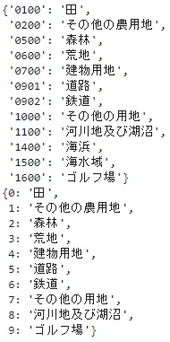
土壌分類のマスタを作成。
# 土壌分類のマスタ作成
'''
https://nlftp.mlit.go.jp/ksj/gml/codelist/LandUseCd-09.html

0100	田	湿田・乾田・沼田・蓮田及び田とする。
0200	その他の農用地	麦・陸稲・野菜・草地・芝地・りんご・梨・桃・ブドウ・茶・桐・はぜ・こうぞ・しゅろ等を栽培する土地とする。
0300	-	-
0400	-	-
0500	森林	多年生植物の密生している地域とする。
0600	荒地	しの地・荒地・がけ・岩・万年雪・湿地・採鉱地等で旧土地利用データが荒地であるところとする。
0700	建物用地	住宅地・市街地等で建物が密集しているところとする。
0800	-	-
0901	道路	道路などで、面的に捉えられるものとする。
0902	鉄道	鉄道・操車場などで、面的にとらえられるものとする。
1000	その他の用地	運動競技場、空港、競馬場・野球場・学校・港湾地区・人工造成地の空地等とする。
1100	河川地及び湖沼	人工湖・自然湖・池・養魚場等で平水時に常に水を湛えているところ及び河川・河川区域の河川敷とする。
1200	-	-
1300	-	-
1400	海浜	海岸に接する砂、れき、岩の区域とする。
1500	海水域	隠顕岩、干潟、シーパースも海に含める。
1600	ゴルフ場	ゴルフ場のゴルフコースの集まっている部分のフェアウエイ及びラフの外側と森林の境目を境界とする。
'''
area_use_categories = {'0100':'田', '0200':'その他の農用地', '0500':'森林', '0600':'荒地', '0700':'建物用地', '0901':'道路'
                       , '0902':'鉄道', '1000':'その他の用地', '1100':'河川地及び湖沼', '1400':'海浜', '1500':'海水域', '1600':'ゴルフ場'
                      }
area_use_categories_le = {j:area_use_categories[i] for i, j in zip(le.classes_, le.transform(le.classes_))}
display(area_use_categories)
display(area_use_categories_le)
土壌分類データを可視化してみる。
# 試しにベクターデータを可視化
plt.rcParams['font.family'] = prop.get_name() #全体のフォントを設定
fig = plt.figure(figsize=(7, 3))
ax = plt.subplot(1,3,1)
re_shape_tsukuba_mirai_2RasterCrs.plot(facecolor='None', ax=ax, edgecolor='k', linewidth=0.3)
plt.setp(ax.get_xticklabels(), fontsize=4)
plt.setp(ax.get_yticklabels(), fontsize=4)
ax.yaxis.offsetText.set_fontsize(4)
ax.yaxis.set_major_formatter(ptick.ScalarFormatter(useMathText=True))
ax.ticklabel_format(style='sci', axis='y', scilimits=(0,0))
ax.grid(False)
# 一部だけグラウンドトゥルースプロット
ax = plt.subplot(1,3,2)
re_shape_tsukuba_mirai_2RasterCrs.plot(facecolor='None', ax=ax, edgecolor='k', linewidth=0.3)
divider = mpl_toolkits.axes_grid1.make_axes_locatable(ax)
cax = divider.append_axes('right', '5%', pad='3%')
ground_truth_2RasterCrs_concat_crop_exploded.sample(2000).plot(column='le_L03b_002', facecolor='pink', ax=ax, edgecolor='k', linewidth=0.05, cmap='tab10', legend=True, cax=cax)
plt.setp(ax.get_xticklabels(), fontsize=4)
plt.setp(ax.get_yticklabels(), fontsize=4)
ax.yaxis.offsetText.set_fontsize(4)
ax.yaxis.set_major_formatter(ptick.ScalarFormatter(useMathText=True))
ax.ticklabel_format(style='sci', axis='y', scilimits=(0,0))
ax.grid(False)
cax.tick_params(labelsize='4')
cax.set_yticks([c for c in area_use_categories_le.keys()])
cax.set_yticklabels([c for c in area_use_categories_le.values()])
# グラウンドトゥルースプロット
ax = plt.subplot(1,3,3)
re_shape_tsukuba_mirai_2RasterCrs.plot(facecolor='None', ax=ax)
divider = mpl_toolkits.axes_grid1.make_axes_locatable(ax)
cax = divider.append_axes('right', '5%', pad='3%')
img = ground_truth_2RasterCrs_concat_crop_exploded.iloc[:,:].plot(column='le_L03b_002', facecolor='lightpink', ax=ax, edgecolor='k', linewidth=0.05, cmap='tab10', legend=True, cax=cax)
plt.setp(ax.get_xticklabels(), fontsize=4)
plt.setp(ax.get_yticklabels(), fontsize=4)
ax.yaxis.offsetText.set_fontsize(4)
ax.yaxis.set_major_formatter(ptick.ScalarFormatter(useMathText=True))
ax.ticklabel_format(style='sci', axis='y', scilimits=(0,0))
ax.grid(False)
cax.tick_params(labelsize='4')
cax.set_yticks([c for c in area_use_categories_le.keys()])
cax.set_yticklabels([c for c in area_use_categories_le.values()])
plt.tight_layout()
plt.show()
左から、小地域境界データのみ可視化、土壌分類データの一部をサンプリングして可視化、土壌分類データすべてを可視化。
細かく土壌が分類されていることが確認できる。
つくばみらい市の土壌種類は10種存在していた。水田多いなー。米所だな。

バンド演算
前処理済みの衛星データファイルリストを取得。
# 各バンドのtifファイルのリスト
B04s_resampling = sorted(list(glob.glob(os.path.join(s2Output,'resampling_S2*B04_crop.tif*'))), key=lambda x:(x.split('_54SVE_')[-1]))
B08s_resampling = sorted(list(glob.glob(os.path.join(s2Output,'resampling_S2*B08_crop.tif*'))), key=lambda x:(x.split('_54SVE_')[-1]))
B11s_resampling = sorted(list(glob.glob(os.path.join(s2Output,'resampling_S2*B11_crop.tif*'))), key=lambda x:(x.split('_54SVE_')[-1]))
B12s_resampling = sorted(list(glob.glob(os.path.join(s2Output,'resampling_S2*B12_crop.tif*'))), key=lambda x:(x.split('_54SVE_')[-1]))

B03s_resampling = sorted(list(glob.glob(os.path.join(s2Output,'resampling_S2*B03_crop.tif*'))), key=lambda x:(x.split('_54SVE_')[-1]))
B02s_resampling = sorted(list(glob.glob(os.path.join(s2Output,'resampling_S2*B02_crop.tif*'))), key=lambda x:(x.split('_54SVE_')[-1]))
print(B04s_resampling)
print(B08s_resampling)
print(B11s_resampling)
print(B12s_resampling)
print(B03s_resampling)
print(B02s_resampling)

バンド演算による指数は11種計算した。
それぞれ、NDBI(正規化都市化指数)、UI(都市化指数)、NDVI(正規化植生指数)、GNDVI(Green正規化植生指数)、BA(都市域)、MSAVI2(修正土壌調整植生指数)、MNDWI(修正正規化水指数)、NDWI(正規化水指数)、NDSI(正規化土壌指数)、BSI(裸地化指数)、DBSI(乾燥裸地指数)である。
あまり指標の知識に明るくないので、上記の指数は以下のような文献に書いてあるものをピックアップした。
- [書籍]基礎からわかるリモートセンシング
- esri 指数ギャラリー
- [PDF file]時系列LANDSATデータによる足尾荒廃山地における植生回復モニタリング
- (研究成果) 水田の代かき時期を衛星データで広域把握 用語の解説:MNDWI
- [PDF file]尾瀬地域における衛星リモートセンシングによる植生モニタリング手法の検討
- [PDF file]植物群落内放射伝達モデルを用いたマルチスペクトルカメラの違いによる水田観測結果への影響評価
- [PDF file]Impervious Surface Extraction by Linear Spectral Mixture Analysis with Post-Processing Model
- [PDF file]Developing soil indices based on brightness, darkness, and greenness to improve land surface mapping accuracy
これら指数はすべて、バンド2,3,4,8,11,12の6種から計算できる。
バンド演算し、可視化してTIFファイルとして保存する。
# バンド演算し、可視化&TIFファイルとして保存
fig = plt.figure(figsize=(12, 16))
for num, (b04, b08, b11, b12, b03, b02) in enumerate(zip(B04s_resampling, B08s_resampling, B11s_resampling, B12s_resampling, B03s_resampling, B02s_resampling)):
    print('#####', os.path.basename(b08).split('_')[3], '#####')
    riod04_resampling = rio.open(b04).read()  # Red
    riod08_resampling = rio.open(b08).read()  # NIR
    riod11 = rio.open(b11)
    riod11_resampling = riod11.read()  # SWIR1
    riod12 = rio.open(b12)
    riod12_resampling = riod12.read()  # SWIR2
    riod03_resampling = rio.open(b03).read()  # Green
    riod02_resampling = rio.open(b02).read()  # Blue
    bounds = riod11.bounds
    print(riod04_resampling.shape)
    print(riod08_resampling.shape)
    print(riod11_resampling.shape)
    print(riod12_resampling.shape)
    print(riod03_resampling.shape)
    print(riod02_resampling.shape)

    # 可視近赤外(VNIR)、短波長赤外(SWIR)、熱赤外(TIR)、近赤外(NRI)
    # NDBI = SWIR1(Band11)-NIR(Band8) / SWIR1(Band11)+NIR(Band8)  正規化都市化指数
    # UI = ((SWIR2 - NIR) / (SWIR2 + NIR))  都市化指数
    # NDVI = NIR(Band8) - RED(Band4) / NIR(Band8) + RED(Band4)  正規化植生指数
    # GNDVI = ( NIR - Green) / ( NIR + Green)  Green正規化植生指数
    # BA = NDBI - NDVI  都市域
    # MSAVI2 = (1/2)*(2(NIR+1)-sqrt((2*NIR+1)^2-8(NIR-Red)))  修正土壌調整植生指数
      # SAVI(土壌調整係数を使用して、土壌の明るさの影響を最小限に抑えることを目的とした植生指数)での露出土壌の影響を最小限に抑えることを目的とした植生指数
    # MNDWI = (Green - SWIR) / (Green + SWIR)  修正正規化水指数
    # NDWI = (NIR-SWIR) / (NIR+SWIR)  正規化水指数
    # NDSI = (SWIR2 - Green) / (SWIR2 + Green)  正規化土壌指数
    # BSI = (SWIR1+Green)-(NIR+Blue) / (SWIR1+Green)+(NIR+Blue)  裸地化指数
    # DBSI =( (SWIR1 − GREEN) / (SWIR1 + GREEN) ) − NDVI  乾燥裸地指数
    NDBI = ( riod11_resampling.astype(float) - riod08_resampling.astype(float) ) / ( riod11_resampling.astype(float) + riod08_resampling.astype(float) )
    UI = ( riod12_resampling.astype(float) - riod08_resampling.astype(float) ) / ( riod12_resampling.astype(float) + riod08_resampling.astype(float) )
    NDVI = ( riod08_resampling.astype(float) - riod04_resampling.astype(float) ) / ( riod08_resampling.astype(float) + riod04_resampling.astype(float) )
    GNDVI = ( riod08_resampling.astype(float) - riod03_resampling.astype(float) ) / ( riod08_resampling.astype(float) + riod03_resampling.astype(float) )
    BA = NDBI - NDVI
    MSAVI2 = (1/2)*( 2*(riod08_resampling.astype(float)+1) - np.sqrt( (2*riod08_resampling.astype(float)+1)**2 - 8*(riod08_resampling.astype(float)-riod04_resampling.astype(float)) ) )
    MNDWI = (riod03_resampling.astype(float) - riod11_resampling.astype(float)) / (riod03_resampling.astype(float) + riod11_resampling.astype(float))
    NDWI = (riod04_resampling.astype(float) - riod11_resampling.astype(float)) / (riod04_resampling.astype(float) + riod11_resampling.astype(float))
    NDSI = ( riod12_resampling.astype(float) - riod03_resampling.astype(float) ) / ( riod12_resampling.astype(float) + riod03_resampling.astype(float) )
    BSI = ( (riod11_resampling.astype(float) + riod03_resampling.astype(float)) - (riod08_resampling.astype(float) + riod02_resampling.astype(float)) ) / ( (riod11_resampling.astype(float) + riod03_resampling.astype(float)) + (riod08_resampling.astype(float) + riod02_resampling.astype(float)) )
    DBSI = ( ( riod11_resampling.astype(float) - riod03_resampling.astype(float) ) / ( riod11_resampling.astype(float) + riod03_resampling.astype(float) ) ) - NDVI

    # NDBI可視化
    ax = plt.subplot(11,6,num+1)
    img = ax.imshow(NDBI[0], cmap='coolwarm', vmin=np.quantile(NDBI[0], q=0.01), vmax=np.quantile(NDBI[0], q=0.99), extent=[bounds.left, bounds.right, bounds.bottom, bounds.top])
    plt.setp(ax.get_xticklabels(), fontsize=4)
    plt.setp(ax.get_yticklabels(), fontsize=4)
    divider = mpl_toolkits.axes_grid1.make_axes_locatable(ax)
    cax = divider.append_axes('right', '5%', pad='3%')
    cbar = plt.colorbar(img, cax=cax)
    cbar.ax.tick_params(labelsize=4)
    ax.set_title('NDBI_'+os.path.basename(riod11.name).split('_')[3]+'_'+os.path.basename(riod11.name).split('_')[6], fontsize=4)
    re_shape_tsukuba_mirai_2RasterCrs.plot(facecolor='none', edgecolor='k', alpha=0.5, ax=ax, linewidth=0.5)
    ax.yaxis.offsetText.set_fontsize(4)
    ax.yaxis.set_major_formatter(ptick.ScalarFormatter(useMathText=True))
    ax.ticklabel_format(style='sci', axis='y', scilimits=(0,0))
    ax.grid(False)

    # UI可視化
    ax = plt.subplot(11,6,num+1+6)
    img = ax.imshow(UI[0], cmap='coolwarm', vmin=np.quantile(UI[0], q=0.01), vmax=np.quantile(UI[0], q=0.99), extent=[bounds.left, bounds.right, bounds.bottom, bounds.top])
    plt.setp(ax.get_xticklabels(), fontsize=4)
    plt.setp(ax.get_yticklabels(), fontsize=4)
    divider = mpl_toolkits.axes_grid1.make_axes_locatable(ax)
    cax = divider.append_axes('right', '5%', pad='3%')
    cbar = plt.colorbar(img, cax=cax)
    cbar.ax.tick_params(labelsize=4)
    ax.set_title('UI_'+os.path.basename(riod11.name).split('_')[3]+'_'+os.path.basename(riod11.name).split('_')[6], fontsize=4)
    re_shape_tsukuba_mirai_2RasterCrs.plot(facecolor='none', edgecolor='k', alpha=0.5, ax=ax, linewidth=0.5)
    ax.yaxis.offsetText.set_fontsize(4)
    ax.yaxis.set_major_formatter(ptick.ScalarFormatter(useMathText=True))
    ax.ticklabel_format(style='sci', axis='y', scilimits=(0,0))
    ax.grid(False)

    # BA可視化
    ax = plt.subplot(11,6,num+1+12)
    img = ax.imshow(BA[0], cmap='RdBu_r', vmin=np.quantile(BA[0], q=0.01), vmax=np.quantile(BA[0], q=0.99), extent=[bounds.left, bounds.right, bounds.bottom, bounds.top])
    plt.setp(ax.get_xticklabels(), fontsize=4)
    plt.setp(ax.get_yticklabels(), fontsize=4)
    divider = mpl_toolkits.axes_grid1.make_axes_locatable(ax)
    cax = divider.append_axes('right', '5%', pad='3%')
    cbar = plt.colorbar(img, cax=cax)
    cbar.ax.tick_params(labelsize=4)
    ax.set_title('BA_'+os.path.basename(riod11.name).split('_')[3]+'_'+os.path.basename(riod11.name).split('_')[6], fontsize=4)
    re_shape_tsukuba_mirai_2RasterCrs.plot(facecolor='none', edgecolor='k', alpha=0.5, ax=ax, linewidth=0.5)
    ax.yaxis.offsetText.set_fontsize(4)
    ax.yaxis.set_major_formatter(ptick.ScalarFormatter(useMathText=True))
    ax.ticklabel_format(style='sci', axis='y', scilimits=(0,0))
    ax.grid(False)

    # NDVI可視化
    ax = plt.subplot(11,6,num+1+18)
    img = ax.imshow(NDVI[0], cmap='RdYlGn', vmin=np.quantile(NDVI[0], q=0.01), vmax=np.quantile(NDVI[0], q=0.99), extent=[bounds.left, bounds.right, bounds.bottom, bounds.top])
    plt.setp(ax.get_xticklabels(), fontsize=4)
    plt.setp(ax.get_yticklabels(), fontsize=4)
    divider = mpl_toolkits.axes_grid1.make_axes_locatable(ax)
    cax = divider.append_axes('right', '5%', pad='3%')
    cbar = plt.colorbar(img, cax=cax)
    cbar.ax.tick_params(labelsize=4)
    ax.set_title('NDVI_'+os.path.basename(riod11.name).split('_')[3]+'_'+os.path.basename(riod11.name).split('_')[6], fontsize=4)
    re_shape_tsukuba_mirai_2RasterCrs.plot(facecolor='none', edgecolor='k', alpha=0.5, ax=ax, linewidth=0.5)
    ax.yaxis.offsetText.set_fontsize(4)
    ax.yaxis.set_major_formatter(ptick.ScalarFormatter(useMathText=True))
    ax.ticklabel_format(style='sci', axis='y', scilimits=(0,0))
    ax.grid(False)

    # GNDVI可視化
    ax = plt.subplot(11,6,num+1+24)
    img = ax.imshow(GNDVI[0], cmap='RdYlGn', vmin=np.quantile(GNDVI[0], q=0.01), vmax=np.quantile(GNDVI[0], q=0.99), extent=[bounds.left, bounds.right, bounds.bottom, bounds.top])
    plt.setp(ax.get_xticklabels(), fontsize=4)
    plt.setp(ax.get_yticklabels(), fontsize=4)
    divider = mpl_toolkits.axes_grid1.make_axes_locatable(ax)
    cax = divider.append_axes('right', '5%', pad='3%')
    cbar = plt.colorbar(img, cax=cax)
    cbar.ax.tick_params(labelsize=4)
    ax.set_title('GNDVI_'+os.path.basename(riod11.name).split('_')[3]+'_'+os.path.basename(riod11.name).split('_')[6], fontsize=4)
    re_shape_tsukuba_mirai_2RasterCrs.plot(facecolor='none', edgecolor='k', alpha=0.5, ax=ax, linewidth=0.5)
    ax.yaxis.offsetText.set_fontsize(4)
    ax.yaxis.set_major_formatter(ptick.ScalarFormatter(useMathText=True))
    ax.ticklabel_format(style='sci', axis='y', scilimits=(0,0))
    ax.grid(False)

    # MSAVI2可視化
    ax = plt.subplot(11,6,num+1+30)
    img = ax.imshow(MSAVI2[0], cmap='RdYlGn', vmin=np.quantile(MSAVI2[0], q=0.01), vmax=np.quantile(MSAVI2[0], q=0.99), extent=[bounds.left, bounds.right, bounds.bottom, bounds.top])
    plt.setp(ax.get_xticklabels(), fontsize=4)
    plt.setp(ax.get_yticklabels(), fontsize=4)
    divider = mpl_toolkits.axes_grid1.make_axes_locatable(ax)
    cax = divider.append_axes('right', '5%', pad='3%')
    cbar = plt.colorbar(img, cax=cax)
    cbar.ax.tick_params(labelsize=4)
    ax.set_title('MSAVI2_'+os.path.basename(riod11.name).split('_')[3]+'_'+os.path.basename(riod11.name).split('_')[6], fontsize=4)
    re_shape_tsukuba_mirai_2RasterCrs.plot(facecolor='none', edgecolor='k', alpha=0.5, ax=ax, linewidth=0.5)
    ax.yaxis.offsetText.set_fontsize(4)
    ax.yaxis.set_major_formatter(ptick.ScalarFormatter(useMathText=True))
    ax.ticklabel_format(style='sci', axis='y', scilimits=(0,0))
    ax.grid(False)

    # MNDWI可視化
    ax = plt.subplot(11,6,num+1+36)
    img = ax.imshow(MNDWI[0], cmap='Blues', vmin=np.quantile(MNDWI[0], q=0.01), vmax=np.quantile(MNDWI[0], q=0.99), extent=[bounds.left, bounds.right, bounds.bottom, bounds.top])
    plt.setp(ax.get_xticklabels(), fontsize=4)
    plt.setp(ax.get_yticklabels(), fontsize=4)
    divider = mpl_toolkits.axes_grid1.make_axes_locatable(ax)
    cax = divider.append_axes('right', '5%', pad='3%')
    cbar = plt.colorbar(img, cax=cax)
    cbar.ax.tick_params(labelsize=4)
    ax.set_title('MNDWI_'+os.path.basename(riod11.name).split('_')[3]+'_'+os.path.basename(riod11.name).split('_')[6], fontsize=4)
    re_shape_tsukuba_mirai_2RasterCrs.plot(facecolor='none', edgecolor='k', alpha=0.5, ax=ax, linewidth=0.5)
    ax.yaxis.offsetText.set_fontsize(4)
    ax.yaxis.set_major_formatter(ptick.ScalarFormatter(useMathText=True))
    ax.ticklabel_format(style='sci', axis='y', scilimits=(0,0))
    ax.grid(False)

    # NDWI可視化
    ax = plt.subplot(11,6,num+1+42)
    img = ax.imshow(NDWI[0], cmap='Blues', vmin=np.quantile(NDWI[0], q=0.01), vmax=np.quantile(NDWI[0], q=0.99), extent=[bounds.left, bounds.right, bounds.bottom, bounds.top])
    plt.setp(ax.get_xticklabels(), fontsize=4)
    plt.setp(ax.get_yticklabels(), fontsize=4)
    divider = mpl_toolkits.axes_grid1.make_axes_locatable(ax)
    cax = divider.append_axes('right', '5%', pad='3%')
    cbar = plt.colorbar(img, cax=cax)
    cbar.ax.tick_params(labelsize=4)
    ax.set_title('NDWI_'+os.path.basename(riod11.name).split('_')[3]+'_'+os.path.basename(riod11.name).split('_')[6], fontsize=4)
    re_shape_tsukuba_mirai_2RasterCrs.plot(facecolor='none', edgecolor='k', alpha=0.5, ax=ax, linewidth=0.5)
    ax.yaxis.offsetText.set_fontsize(4)
    ax.yaxis.set_major_formatter(ptick.ScalarFormatter(useMathText=True))
    ax.ticklabel_format(style='sci', axis='y', scilimits=(0,0))
    ax.grid(False)

    # NDSI可視化
    ax = plt.subplot(11,6,num+1+48)
    img = ax.imshow(NDSI[0], cmap='PuOr_r', vmin=np.quantile(NDSI[0], q=0.01), vmax=np.quantile(NDSI[0], q=0.99), extent=[bounds.left, bounds.right, bounds.bottom, bounds.top])
    plt.setp(ax.get_xticklabels(), fontsize=4)
    plt.setp(ax.get_yticklabels(), fontsize=4)
    divider = mpl_toolkits.axes_grid1.make_axes_locatable(ax)
    cax = divider.append_axes('right', '5%', pad='3%')
    cbar = plt.colorbar(img, cax=cax)
    cbar.ax.tick_params(labelsize=4)
    ax.set_title('NDSI_'+os.path.basename(riod11.name).split('_')[3]+'_'+os.path.basename(riod11.name).split('_')[6], fontsize=4)
    re_shape_tsukuba_mirai_2RasterCrs.plot(facecolor='none', edgecolor='k', alpha=0.5, ax=ax, linewidth=0.5)
    ax.yaxis.offsetText.set_fontsize(4)
    ax.yaxis.set_major_formatter(ptick.ScalarFormatter(useMathText=True))
    ax.ticklabel_format(style='sci', axis='y', scilimits=(0,0))
    ax.grid(False)

    # BSI可視化
    ax = plt.subplot(11,6,num+1+54)
    img = ax.imshow(BSI[0], cmap='PuOr_r', vmin=np.quantile(BSI[0], q=0.01), vmax=np.quantile(BSI[0], q=0.99), extent=[bounds.left, bounds.right, bounds.bottom, bounds.top])
    plt.setp(ax.get_xticklabels(), fontsize=4)
    plt.setp(ax.get_yticklabels(), fontsize=4)
    divider = mpl_toolkits.axes_grid1.make_axes_locatable(ax)
    cax = divider.append_axes('right', '5%', pad='3%')
    cbar = plt.colorbar(img, cax=cax)
    cbar.ax.tick_params(labelsize=4)
    ax.set_title('BSI_'+os.path.basename(riod11.name).split('_')[3]+'_'+os.path.basename(riod11.name).split('_')[6], fontsize=4)
    re_shape_tsukuba_mirai_2RasterCrs.plot(facecolor='none', edgecolor='k', alpha=0.5, ax=ax, linewidth=0.5)
    ax.yaxis.offsetText.set_fontsize(4)
    ax.yaxis.set_major_formatter(ptick.ScalarFormatter(useMathText=True))
    ax.ticklabel_format(style='sci', axis='y', scilimits=(0,0))
    ax.grid(False)

    # DBSI可視化
    ax = plt.subplot(11,6,num+1+60)
    img = ax.imshow(DBSI[0], cmap='PuOr_r', vmin=np.quantile(DBSI[0], q=0.01), vmax=np.quantile(DBSI[0], q=0.99), extent=[bounds.left, bounds.right, bounds.bottom, bounds.top])
    plt.setp(ax.get_xticklabels(), fontsize=4)
    plt.setp(ax.get_yticklabels(), fontsize=4)
    divider = mpl_toolkits.axes_grid1.make_axes_locatable(ax)
    cax = divider.append_axes('right', '5%', pad='3%')
    cbar = plt.colorbar(img, cax=cax)
    cbar.ax.tick_params(labelsize=4)
    ax.set_title('DBSI_'+os.path.basename(riod11.name).split('_')[3]+'_'+os.path.basename(riod11.name).split('_')[6], fontsize=4)
    re_shape_tsukuba_mirai_2RasterCrs.plot(facecolor='none', edgecolor='k', alpha=0.5, ax=ax, linewidth=0.5)
    ax.yaxis.offsetText.set_fontsize(4)
    ax.yaxis.set_major_formatter(ptick.ScalarFormatter(useMathText=True))
    ax.ticklabel_format(style='sci', axis='y', scilimits=(0,0))
    ax.grid(False)

    out_meta = riod11.meta
    out_meta.update({'dtype':rio.float32})
    fname = 'NDBI_'+os.path.basename(riod11.name)
    print(fname)
    with rio.open(os.path.join(s2Output, fname), "w", **out_meta) as dest:
        dest.write(NDBI.astype(rio.float32))

    out_meta = riod11.meta
    out_meta.update({'dtype':rio.float32})
    fname = 'UI_'+os.path.basename(riod11.name)
    print(fname)
    with rio.open(os.path.join(s2Output, fname), "w", **out_meta) as dest:
        dest.write(UI.astype(rio.float32))

    out_meta = riod11.meta
    out_meta.update({'dtype':rio.float32})
    fname = 'BA_'+os.path.basename(riod11.name)
    print(fname)
    with rio.open(os.path.join(s2Output, fname), "w", **out_meta) as dest:
        dest.write(BA.astype(rio.float32))

    out_meta = riod11.meta
    out_meta.update({'dtype':rio.float32})
    fname = 'NDVI_'+os.path.basename(riod11.name)
    print(fname)
    with rio.open(os.path.join(s2Output, fname), "w", **out_meta) as dest:
        dest.write(NDVI.astype(rio.float32))

    out_meta = riod11.meta
    out_meta.update({'dtype':rio.float32})
    fname = 'GNDVI_'+os.path.basename(riod11.name)
    print(fname)
    with rio.open(os.path.join(s2Output, fname), "w", **out_meta) as dest:
        dest.write(GNDVI.astype(rio.float32))

    out_meta = riod11.meta
    out_meta.update({'dtype':rio.float32})
    fname = 'MSAVI2_'+os.path.basename(riod11.name)
    print(fname)
    with rio.open(os.path.join(s2Output, fname), "w", **out_meta) as dest:
        dest.write(MSAVI2.astype(rio.float32))

    out_meta = riod11.meta
    out_meta.update({'dtype':rio.float32})
    fname = 'MNDWI_'+os.path.basename(riod11.name)
    print(fname)
    with rio.open(os.path.join(s2Output, fname), "w", **out_meta) as dest:
        dest.write(MNDWI.astype(rio.float32))

    out_meta = riod11.meta
    out_meta.update({'dtype':rio.float32})
    fname = 'NDWI_'+os.path.basename(riod11.name)
    print(fname)
    with rio.open(os.path.join(s2Output, fname), "w", **out_meta) as dest:
        dest.write(NDWI.astype(rio.float32))

    out_meta = riod11.meta
    out_meta.update({'dtype':rio.float32})
    fname = 'NDSI_'+os.path.basename(riod11.name)
    print(fname)
    with rio.open(os.path.join(s2Output, fname), "w", **out_meta) as dest:
        dest.write(NDSI.astype(rio.float32))

    out_meta = riod11.meta
    out_meta.update({'dtype':rio.float32})
    fname = 'BSI_'+os.path.basename(riod11.name)
    print(fname)
    with rio.open(os.path.join(s2Output, fname), "w", **out_meta) as dest:
        dest.write(BSI.astype(rio.float32))

    out_meta = riod11.meta
    out_meta.update({'dtype':rio.float32})
    fname = 'DBSI_'+os.path.basename(riod11.name)
    print(fname,'\n')
    with rio.open(os.path.join(s2Output, fname), "w", **out_meta) as dest:
        dest.write(DBSI.astype(rio.float32))

plt.tight_layout()
plt.show()

保存したTIFファイルリストを取得。
この後は2020年のデータだけを使用していく。
# 各バンドのtifファイルのリスト
NDBI_band_path_list_nomask = sorted(list(glob.glob(os.path.join(s2Output,'NDBI_resampling_S2*.tif*'))), key=lambda x:(x.split('_54SVE_')[-1]))
UI_band_path_list_nomask = sorted(list(glob.glob(os.path.join(s2Output,'UI_resampling_S2*.tif*'))), key=lambda x:(x.split('_54SVE_')[-1]))
BA_band_path_list_nomask = sorted(list(glob.glob(os.path.join(s2Output,'BA_resampling_S2*.tif*'))), key=lambda x:(x.split('_54SVE_')[-1]))
NDVI_band_path_list_nomask = sorted(list(glob.glob(os.path.join(s2Output,'NDVI_resampling_S2*.tif*'))), key=lambda x:(x.split('_54SVE_')[-1]))
GNDVI_band_path_list_nomask = sorted(list(glob.glob(os.path.join(s2Output,'GNDVI_resampling_S2*.tif*'))), key=lambda x:(x.split('_54SVE_')[-1]))
MSAVI2_band_path_list_nomask = sorted(list(glob.glob(os.path.join(s2Output,'MSAVI2_resampling_S2*.tif*'))), key=lambda x:(x.split('_54SVE_')[-1]))
MNDWI_band_path_list_nomask = sorted(list(glob.glob(os.path.join(s2Output,'MNDWI_resampling_S2*.tif*'))), key=lambda x:(x.split('_54SVE_')[-1]))
NDWI_band_path_list_nomask = sorted(list(glob.glob(os.path.join(s2Output,'NDWI_resampling_S2*.tif*'))), key=lambda x:(x.split('_54SVE_')[-1]))
NDSI_band_path_list_nomask = sorted(list(glob.glob(os.path.join(s2Output,'NDSI_resampling_S2*.tif*'))), key=lambda x:(x.split('_54SVE_')[-1]))
BSI_band_path_list_nomask = sorted(list(glob.glob(os.path.join(s2Output,'BSI_resampling_S2*.tif*'))), key=lambda x:(x.split('_54SVE_')[-1]))
DBSI_band_path_list_nomask = sorted(list(glob.glob(os.path.join(s2Output,'DBSI_resampling_S2*.tif*'))), key=lambda x:(x.split('_54SVE_')[-1]))
band_paths_list = NDBI_band_path_list_nomask + UI_band_path_list_nomask + BA_band_path_list_nomask + NDVI_band_path_list_nomask + GNDVI_band_path_list_nomask + MSAVI2_band_path_list_nomask + MNDWI_band_path_list_nomask + NDWI_band_path_list_nomask + NDSI_band_path_list_nomask + BSI_band_path_list_nomask + DBSI_band_path_list_nomask
rio_file_list2020 = band_paths_list[2:][::6]
display(rio_file_list2020)

rasterstats.zonal_statsを使って、土壌分類のベクターファイルの各Polygon内でバンド演算した各指標の平均値を計算し、バンド演算のTIFファイルをベクターデータ化する。
# 土壌分類のベクターファイルのPolygon内のバンド演算指標の平均値を計算して、TIFファイルをベクターファイル化
def add_stats_vals(rio_data, vec_data, add_col_name, area_col='S_NAME'):
    affine = rio_data.transform
    mean_stats = rasterstats.zonal_stats(vec_data, rio_data.read(1)
                                         , affine=affine
                                         , add_stats={'mymean':lambda x: np.ma.mean(x)}) # np.ma.filled(x, fill_value=np.nan)
    mean_stats = [m['mymean'] for m in mean_stats]  # 平均値を取得
    vec_data_stats = vec_data#.copy()
    vec_data_stats[add_col_name] = mean_stats
    vec_data_stats[add_col_name] = vec_data_stats[add_col_name].map(lambda x: np.ma.filled(x, fill_value=np.nan))  # Maskの箇所はnanに変更
    # 欠損値は小地域ごとの平均値で埋める
    category_means = vec_data_stats.dropna(subset=[add_col_name]).groupby(area_col)[add_col_name].mean()  # カテゴリごとの平均を計算
    vec_data_stats[add_col_name] = vec_data_stats[add_col_name].fillna(vec_data_stats[area_col].map(category_means))
    return vec_data_stats

if DOWNLOAD:
    ground_truth_2RasterCrs_concat_crop_exploded_stats = ground_truth_2RasterCrs_concat_crop_exploded.copy()
    for riofile in rio_file_list2020:
        riodata = rio.open(riofile)
        ground_truth_2RasterCrs_concat_crop_exploded_stats = add_stats_vals(riodata
                                                                            , ground_truth_2RasterCrs_concat_crop_exploded_stats
                                                                            , os.path.basename(riofile).split('_')[0]+'_mean'
                                                                            , area_col='S_NAME')
    ground_truth_2RasterCrs_concat_crop_exploded_stats.to_file(os.path.join(shape_path, "ground_truth_2RasterCrs_concat_crop_exploded_stats.shp"), encoding="shift-jis")
    display(ground_truth_2RasterCrs_concat_crop_exploded_stats)

# SHAPEファイルのカラム名は10文字以内の制限があるので、"MSAVI2_mean"は"MSAVI2_mea"になってしまっている
ground_truth_2RasterCrs_concat_crop_exploded_stats = gpd.read_file(os.path.join(shape_path, "ground_truth_2RasterCrs_concat_crop_exploded_stats.shp"), encoding="shift-jis")
ground_truth_2RasterCrs_concat_crop_exploded_stats.rename(columns={'MSAVI2_mea':'MSAVI2_mean'}, inplace=True)
ground_truth_2RasterCrs_concat_crop_exploded_stats.rename(columns={'le_L03b_00':'le_L03b_002'}, inplace=True)
display(ground_truth_2RasterCrs_concat_crop_exploded_stats)

バンド演算のラスターデータ、バンド演算のベクターデータ、土壌分類のベクターデータをプロットしてみる。
ベクターデータ化しても、ラスターデータと同じ傾向が見える。
バンド演算のベクターデータと土壌分類のベクターデータを比較すると、ちゃんと関連もありそう。モデリングもできそうだな。
# バンド演算のラスターデータplot、バンド演算のベクターデータplot、土壌分類plot
fig = plt.figure(figsize=(6, 18))
num = 0
for i, file in tqdm(enumerate(rio_file_list2020)):
    riodata = rio.open(file)
    fname = os.path.basename(file)
    satIndex = fname.split('_')[0]
    if satIndex=='NDBI' or satIndex=='UI' or satIndex=='BA':
        cmap = 'coolwarm'
    elif satIndex=='NDVI' or satIndex=='GNDVI' or satIndex=='MSAVI2':
        cmap = 'RdYlGn'
    elif satIndex=='MNDWI' or satIndex=='NDWI':
        cmap = 'Blues'
    elif satIndex=='NDSI' or satIndex=='BSI' or satIndex=='DBSI':
        cmap = 'PuOr_r'
    else:
        cmap = 'RdYlGn_r'

    ax = plt.subplot(len(rio_file_list2020), 3, num+1)
    divider = mpl_toolkits.axes_grid1.make_axes_locatable(ax)
    retted = show(riodata, ax=ax
                  , vmin=np.quantile(riodata.read(), 0.01)
                  , vmax=np.quantile(riodata.read(), 0.99)
                  , cmap=cmap)
    img = retted.get_images()[0]
    divider = mpl_toolkits.axes_grid1.make_axes_locatable(ax)
    cax = divider.append_axes('right', '5%', pad='3%')
    cbar = plt.colorbar(img, cax=cax)
    cbar.ax.tick_params(labelsize=4, width=0.4, length=5)
    plt.setp(ax.get_xticklabels(), fontsize=4)
    plt.setp(ax.get_yticklabels(), fontsize=4)
    ax.set_title(fname.split('_')[0]+'_'+fname.split('_')[4]+'_RasterMap', fontsize=4)
    re_shape_tsukuba_mirai_2RasterCrs.plot(facecolor='none', edgecolor='k', ax=ax, linewidth=0.2)
    ax.yaxis.offsetText.set_fontsize(4)
    ax.yaxis.set_major_formatter(ptick.ScalarFormatter(useMathText=True))
    ax.ticklabel_format(style='sci', axis='y', scilimits=(0,0))
    ax.grid(False)

    ax = plt.subplot(len(rio_file_list2020), 3, num+2)
    show(riodata, ax=ax
         , vmin=np.quantile(riodata.read(), 0.01)
         , vmax=np.quantile(riodata.read(), 0.99)
         , alpha=0.6, cmap='Greys_r')
    divider = mpl_toolkits.axes_grid1.make_axes_locatable(ax)
    cax = divider.append_axes('right', '5%', pad='3%')
    img = ground_truth_2RasterCrs_concat_crop_exploded_stats.plot(column=satIndex+'_mean', cmap=cmap, edgecolor='k', legend=True, ax=ax, cax=cax
                                                                  , linewidth=0.05
                                                                  , vmin=np.nanquantile(ground_truth_2RasterCrs_concat_crop_exploded_stats[satIndex+'_mean'], 0.01)
                                                                  , vmax=np.nanquantile(ground_truth_2RasterCrs_concat_crop_exploded_stats[satIndex+'_mean'], 0.99)
                                                                  #, alpha=0.6
                                                                 )
    cax.tick_params(labelsize='4', width=0.4, length=5)
    plt.setp(ax.get_xticklabels(), fontsize=4)
    plt.setp(ax.get_yticklabels(), fontsize=4)
    ax.set_title(fname.split('_')[0]+'_'+fname.split('_')[4]+'_VectorMap', fontsize=4)
    # re_shape_tsukuba_mirai_2RasterCrs_NDBI.plot(facecolor='none', edgecolor='k', alpha=0.8, ax=ax, linewidth=0.2)
    ax.yaxis.offsetText.set_fontsize(4)
    ax.yaxis.set_major_formatter(ptick.ScalarFormatter(useMathText=True))
    ax.ticklabel_format(style='sci', axis='y', scilimits=(0,0))
    ax.grid(False)

    ax = plt.subplot(len(rio_file_list2020), 3, num+3)
    show(riodata, ax=ax
         , vmin=np.quantile(riodata.read(), 0.01)
         , vmax=np.quantile(riodata.read(), 0.99)
         , alpha=0.6, cmap='Greys_r')
    divider = mpl_toolkits.axes_grid1.make_axes_locatable(ax)
    cax = divider.append_axes('right', '5%', pad='3%')
    img = ground_truth_2RasterCrs_concat_crop_exploded_stats.plot(column='le_L03b_002', cmap='tab10', edgecolor='k', legend=True, ax=ax, cax=cax
                                                                  , linewidth=0.05
                                                                  #, vmin=np.nanquantile(ground_truth_2RasterCrs_concat_crop_exploded_stats['NDBI_mean'], 0.01)
                                                                  #, vmax=np.nanquantile(ground_truth_2RasterCrs_concat_crop_exploded_stats['NDBI_mean'], 0.99)
                                                                  #, alpha=0.6
                                                                 )
    cax.tick_params(labelsize='4', width=0.4, length=5)
    cax.set_yticks([c for c in area_use_categories_le.keys()])
    cax.set_yticklabels([c for c in area_use_categories_le.values()])
    plt.setp(ax.get_xticklabels(), fontsize=4)
    plt.setp(ax.get_yticklabels(), fontsize=4)
    ax.set_title(fname.split('_')[0]+'_'+fname.split('_')[4]+'_SoilCategory', fontsize=4)
    # re_shape_tsukuba_mirai_2RasterCrs_NDBI.plot(facecolor='none', edgecolor='k', alpha=0.8, ax=ax, linewidth=0.2)
    ax.yaxis.offsetText.set_fontsize(4)
    ax.yaxis.set_major_formatter(ptick.ScalarFormatter(useMathText=True))
    ax.ticklabel_format(style='sci', axis='y', scilimits=(0,0))
    ax.grid(False)
    num += 3

plt.tight_layout()
plt.show()

PolygonをPointに変換する作業を実施。
ちなみにこれはモデリングに必要ない作業だが、一応そのまま実施した履歴として残しておく。
(経緯は、もともとクリギングをしようと思っていた → バリオグラムの計算をする時にPolygonだとエラーが出た(Polygon同士の距離の計算はできないから) → Polygonの地理的重心を使ってPointに変換した → でも結局いい感じのつくばみらい市の連続値のデータを見つけられずクリギングは断念 → Pointに変換した作業は残ったまま)
Pointに変換後、一例としてNDSIのみ可視化。
# PolygonをPointにする
ground_truth_2RasterCrs_concat_crop_exploded_stats_2point = ground_truth_2RasterCrs_concat_crop_exploded_stats.copy()
ground_truth_2RasterCrs_concat_crop_exploded_stats_2point['geometry'] = [p.centroid for p in ground_truth_2RasterCrs_concat_crop_exploded_stats.geometry]

# Point可視化(一例としてNDSIのみ)
satIndex='NDSI'
cmap='PuOr_r'
fig = plt.figure(figsize=(3, 3))
ax = plt.subplot(1,1,1)
divider = mpl_toolkits.axes_grid1.make_axes_locatable(ax)
cax = divider.append_axes('right', '5%', pad='3%')
img = ground_truth_2RasterCrs_concat_crop_exploded_stats_2point.plot(column=satIndex+'_mean', cmap=cmap, edgecolor='k', legend=True, ax=ax, cax=cax
                                                                     , linewidth=0.05, markersize=2
                                                                     , vmin=np.quantile(ground_truth_2RasterCrs_concat_crop_exploded_stats[satIndex+'_mean'], 0.01)
                                                                     , vmax=np.quantile(ground_truth_2RasterCrs_concat_crop_exploded_stats[satIndex+'_mean'], 0.99)
                                                                    )
cax.tick_params(labelsize='4', width=0.4, length=5)
plt.setp(ax.get_xticklabels(), fontsize=4)
plt.setp(ax.get_yticklabels(), fontsize=4)
ax.set_title(satIndex, fontsize=4)
# re_shape_tsukuba_mirai_2RasterCrs_NDBI.plot(facecolor='none', edgecolor='k', alpha=0.8, ax=ax, linewidth=0.2)
ax.yaxis.offsetText.set_fontsize(4)
ax.yaxis.set_major_formatter(ptick.ScalarFormatter(useMathText=True))
ax.ticklabel_format(style='sci', axis='y', scilimits=(0,0))
ax.grid(False)
plt.show()

モデル構築(多項分類)
準備は整ったので、モデリングを実施する。
今回は10種ある土壌の種類を分類するモデルを構築する。
モデルは以下の4種作り、それぞれの結果を見てみる。
- 多項ロジスティック回帰(ソフトマックス回帰)
- ベイズ多項ロジスティック回帰(ソフトマックス回帰)
- 多項ICARモデル
- LightGBM
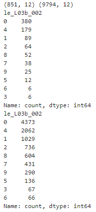
説明変数リストと目的変数を定義して、学習データとテストデータを分けておく。学習データは量が多いと弱小PCではMCMCが回せないので、ある程度少量としておく。(851レコード)
# 説明変数
explanatory_variables = ground_truth_2RasterCrs_concat_crop_exploded_stats_2point.filter(like='mean', axis=1).columns.to_list()
# 目的変数
objective_variables = 'le_L03b_002'

# split data
X_train,X_test,y_train,y_test = sklearn.model_selection.train_test_split(ground_truth_2RasterCrs_concat_crop_exploded_stats_2point[explanatory_variables+['geometry']]
                                                                         , ground_truth_2RasterCrs_concat_crop_exploded_stats_2point[[objective_variables]+['geometry']]
                                                                         , test_size=0.92, shuffle=True, random_state=0
                                                                         , stratify=ground_truth_2RasterCrs_concat_crop_exploded_stats_2point[objective_variables])
print(X_train.shape, X_test.shape)
# 各土壌分類のレコード数
display(y_train[objective_variables].value_counts())
display(y_test[objective_variables].value_counts())
学習データとテストデータの土壌分類の可視化。
# 学習データとテストデータの土壌分類
plt.rcParams['font.family'] = prop.get_name() #全体のフォントを設定
fig = plt.figure(figsize=(6, 3))
ax = plt.subplot(1,2,1)
divider = mpl_toolkits.axes_grid1.make_axes_locatable(ax)
cax = divider.append_axes('right', '5%', pad='3%')
img = y_train.plot(column=objective_variables, cmap='tab10', edgecolor='k', legend=True, ax=ax, cax=cax, linewidth=0.05, markersize=5)
cax.tick_params(labelsize='4', width=0.4, length=5)
plt.setp(ax.get_xticklabels(), fontsize=4)
plt.setp(ax.get_yticklabels(), fontsize=4)
ax.set_title('土壌分類 Point Train', fontsize=4)
re_shape_tsukuba_mirai_2RasterCrs.plot(facecolor='none', edgecolor='k', alpha=0.8, ax=ax, linewidth=0.2)
ax.yaxis.offsetText.set_fontsize(4)
ax.yaxis.set_major_formatter(ptick.ScalarFormatter(useMathText=True))
ax.ticklabel_format(style='sci', axis='y', scilimits=(0,0))
cax.set_yticks([c for c in area_use_categories_le.keys()])
cax.set_yticklabels([c for c in area_use_categories_le.values()])
ax.grid(False)

ax = plt.subplot(1,2,2)
divider = mpl_toolkits.axes_grid1.make_axes_locatable(ax)
cax = divider.append_axes('right', '5%', pad='3%')
img = y_test.plot(column=objective_variables, cmap='tab10', edgecolor='k', legend=True, ax=ax, cax=cax, linewidth=0.05, markersize=1)
cax.tick_params(labelsize='4', width=0.4, length=5)
plt.setp(ax.get_xticklabels(), fontsize=4)
plt.setp(ax.get_yticklabels(), fontsize=4)
ax.set_title('土壌分類 Point Test', fontsize=4)
re_shape_tsukuba_mirai_2RasterCrs.plot(facecolor='none', edgecolor='k', alpha=0.8, ax=ax, linewidth=0.2)
ax.yaxis.offsetText.set_fontsize(4)
ax.yaxis.set_major_formatter(ptick.ScalarFormatter(useMathText=True))
ax.ticklabel_format(style='sci', axis='y', scilimits=(0,0))
cax.set_yticks([c for c in area_use_categories_le.keys()])
cax.set_yticklabels([c for c in area_use_categories_le.values()])
ax.grid(False)
plt.tight_layout()
plt.show()

1. 多項ロジスティック回帰(ソフトマックス回帰)
最初は空間相関を考慮しない単なる多項ロジスティック回帰。scikit-learnで簡単にサクッと実施する。
不均衡データなので、sample weightは設定する。
学習データ、テストデータそれぞれの精度指標結果一覧(classification_report)と混同行列を出力。
F1スコアのマクロ平均を見る感じあまり良いモデルとは言えなそう。
# add sample weight
def sample_w(y_train):
    '''
    output sample weight (balanced weight)
    y_train:True Train data
    '''
    n_samples=len(y_train)
    n_classes=len(np.unique(y_train))
    bincounts = {i:len(y_train[y_train==i]) for i in sorted(np.unique(y_train))}
    class_ratio_param = {key:n_samples / (n_classes * bincnt) for key, bincnt in bincounts.items()}
    #print('class_ratio_param',class_ratio_param)
    sample_weight=np.array([class_ratio_param[r] for r in y_train])
    return sample_weight

# 重みの配列
sample_ws = sample_w(y_train[objective_variables])

# 学習
print(y_train[objective_variables].value_counts(),'\n')
lr = sklearn.linear_model.LogisticRegression(max_iter=1000)
lr.fit(X_train[explanatory_variables], y_train[objective_variables], sample_weight=sample_ws)
result_proba = lr.predict_proba(X_train[explanatory_variables])
result = lr.predict(X_train[explanatory_variables])
reslutDf = pd.DataFrame({'true':y_train[objective_variables].to_numpy(), 'pred':result.ravel()})
print(sklearn.metrics.classification_report(y_train[objective_variables].to_numpy(), result.ravel()),'\n')
cm = sklearn.metrics.confusion_matrix(y_train[objective_variables].to_numpy(), result.ravel())
print(cm,'\n\n######################################\n')

# 未知データに適用
print(y_test[objective_variables].value_counts(),'\n')
result_proba = lr.predict_proba(X_test[explanatory_variables])
result = lr.predict(X_test[explanatory_variables])
reslutDf = pd.DataFrame({'true':y_test[objective_variables].to_numpy(), 'pred':result.ravel()})
print(sklearn.metrics.classification_report(y_test[objective_variables].to_numpy(), result.ravel()),'\n')
cm = sklearn.metrics.confusion_matrix(y_test[objective_variables].to_numpy(), result.ravel())
print(cm)
学習データ
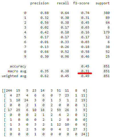
テストデータ

2. ベイズ多項ロジスティック回帰(ソフトマックス回帰)
以前「階層ベイズで個性を捉える(PyMC ver.5.7.2)」という記事でPyMCを使ってベイズモデリングをやってみて楽しかったので、せっかくだからベイズモデリングでも多項ロジスティック回帰をやってみる。
回帰係数と、切片の事前分布は正規分布を仮定、尤度はカテゴリカル対数尤度とする。
クラスの重みを考慮するためにpm.Potentialを使う。pm.Potentialは、モデルの確率密度を調整するために、任意の因子(制約や他の尤度成分など)を追加したりできる。pm.Potentialを使って、対数尤度にクラスの比率に応じた重みをかけて重み付けをする。
with pm.Model() as model:
    # coords(次元やインデックスを定義)
    model.add_coord('data', values=range(X_train.shape[0]), mutable=True)
    model.add_coord('var', values=explanatory_variables, mutable=True)
    model.add_coord('obj_var', values=sorted(y_train[objective_variables].unique()), mutable=True)

    # 説明変数
    x = pm.MutableData('x', X_train[explanatory_variables].to_numpy(), dims=('data', 'var'))
    y = pm.MutableData("y", y_train[objective_variables].to_numpy(), dims=('data', ))
    weights = pm.MutableData("weights", sample_ws, dims=('data', ))

    # 推論パラメータの事前分布
    coef_ = pm.Normal('coef', mu=0.0, sigma=1, dims=("var",'obj_var'))  # 各係数の事前分布は正規分布
    intercept_ = pm.Normal('intercept', mu=0.0, sigma=1.0, dims=("obj_var", ))  # 切片の事前分布は正規分布

    # linear model
    mu = pm.Deterministic("mu", x.dot(coef_)+intercept_, dims=('data', 'obj_var'))
    theta = pm.Deterministic("theta", pm.math.softmax(mu, axis=1), dims=('data', 'obj_var'))  # axis設定しないとダメ

    # 尤度
    #y_pred = pm.Categorical("y_pred", p=theta, observed=y, dims='data')  # 重み付けしない場合
    y_pred = pm.Potential('y_pred', (weights * pm.logp(pm.Categorical.dist(p=theta), y)).sum(axis=0), dims='data')

# モデル構造
modeldag = pm.model_to_graphviz(model)
display(modeldag)

MCMC実行。繰り返し回数は3000、バーンイン期間は1000、チェーンは3つに設定。
%%time
# MCMC実行
# バックエンドでNumPyroで実行
with model:
    # MCMCによる推論
    trace_org = pm.sample(draws=3000, tune=1000, chains=3, nuts_sampler="numpyro", random_seed=1, return_inferencedata=True)
# >> Wall time: 1min 24s
結果を保存。
model_dir = '/content/drive/MyDrive/satelite/model'
os.makedirs(model_dir, exist_ok=True)
# データの保存 to_netcdfの利用
trace_org.to_netcdf(os.path.join(model_dir, 'model_GLM.nc'))

# model_dir = '/content/drive/MyDrive/satelite/model'
# os.makedirs(model_dir, exist_ok=True)
# # データの読み込み from_netcdfの利用
# trace_org = az.from_netcdf(os.path.join(model_dir, 'model_GLM.nc'))
収束を見ていく。
まずは回帰係数と切片のtrace plot。
収束してそう。
# plot_trace
az.plot_trace(trace_org, backend_kwargs={"constrained_layout":True}, var_names=["coef","intercept"])
plt.show()

$\hat{R}$で収束の確認。
$\hat{R}$が1.1を超えているか、超えているならそれはどのパラメータかを出力する。全パラメータの$\hat{R}$の最大値は1.00だったので収束の問題は無さそう。
# MCMCの収束を評価
rhat_vals = az.rhat(trace_org).values()

# 最大のRhatを確認
result = np.max([np.max(i.values) for i in rhat_vals if i.name in ['coef','intercept','mu','theta']])
print('Max rhat:', result)
# 1.1以上のRhatを確認
for i in rhat_vals:
    if np.max(i.values)>=1.1:
        print(i.name, np.max(i.values), np.mean(i.values), i.values.shape, sep='  ====>  ')
# >> Max rhat: 1.0022815343019567
各クラスの事後確率を取り出し、学習データの精度を確認する。
# 各クラスの事後確率theta
softmax_result = pd.DataFrame(trace_org['posterior']['theta'].mean(dim=["chain", "draw"]).values)
y_pred = softmax_result.idxmax(axis=1)
print(sklearn.metrics.classification_report(y_train[objective_variables].to_numpy(), y_pred.ravel()))
cm = sklearn.metrics.confusion_matrix(y_train[objective_variables].to_numpy(), y_pred.ravel())
print(cm)

未知のテストデータへの適用をする時には注意が必要で、pm.Potentialを使うと、pm.sample_posterior_predictiveで事後予測サンプルを生成することができない。(Pm.sample_posterior_predictive() not working with weights)
なので、推定したパラメータを使って、線形モデルを定義して推論してあげる必要がある。
今作ったモデルの場合、パラメータとして回帰係数coefと切片interceptを推定したので、それらを使ってクラスの確率を計算してあげればいい。
クラス数$K=10$、説明変数の数$N=11$、回帰係数$\beta_{n>0,i}$、切片$\beta_{0,i}$として、クラス$i$の確率は以下のように表現できる。
y_{i}=
\frac{e^{\beta_{0,i}+\beta_{1,i}x_{1}+…+\beta_{N,i}x_{N}}}
{\sum_{k=1}^{K} e^{\beta_{0,k}+\beta_{1,k}x_{1}+…+\beta_{N,k}x_{N}}}
上記式を定義して計算してあげるとテストデータの推論が可能になる。
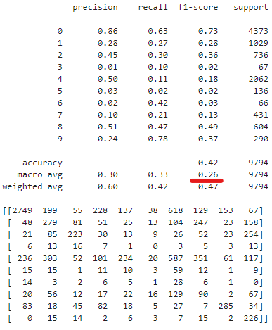
ベイズ推論しているが基本的にさっきのscikit-learnのモデルと同じなので、同じような精度になっていて、F1スコアのマクロ平均を見る感じあまり良いモデルとは言えなそう。
# 未知データへの適用
# 回帰係数の推定値
coefs = trace_org['posterior']['coef'].mean(dim=["chain", "draw"]).values
# 切片の推定値
intercepts = trace_org['posterior']['intercept'].mean(dim=["chain", "draw"]).values
# 線形モデル式
mu = X_test[explanatory_variables].to_numpy().dot(coefs) + intercepts
# ソフトマックス関数に入れる
m = softmax(mu, axis=1)
# 確率が最大のクラスを取得
m_class = m.argmax(axis=1)
# 精度計算
print(sklearn.metrics.classification_report(y_test[objective_variables].to_numpy(), m_class.ravel()))
cm = sklearn.metrics.confusion_matrix(y_test[objective_variables].to_numpy(), m_class.ravel())
print(cm)
3. 多項ICARモデル
Intrinsic CARモデル概要
いよいよ、空間相関を考慮したモデルを作っていく。
まずCARモデルの説明を簡単にしていく。(参考:[書籍]Rではじめる地理空間データの統計解析入門)
CARモデルの最も単純な形は地域特性$z_{i}$と偶発的な要因などを吸収するための誤差項$\epsilon_{i}$だけのモデル。
\displaylines{
y_{i}=z_{i}+\epsilon_{i}
\\
\epsilon_{i} \sim \mathcal{N}(0,\sigma^2)
}
$z_{i}$をどのようにモデル化するかでCARモデルにはバリエーションがあるが、代表的なものにICAR(Intrinsic CAR)モデルがある。このモデルでは$z_{i}$は以下のように定義される。
z_{i}|z_{j{\neq}i} \sim \mathcal{N}(\frac{\sum_{j} \omega_{ij}z_{j}}{\sum_{j} \omega_{ij}}, \frac{\tau^{2}}{\sum_{j} \omega_{ij}})
$z_{i}|z_{j{\neq}i}$は地域$i$以外の地域における変数$z_{j{\neq}i}$で条件づけられた変数$z_{i}$で、他の地域$z_{j{\neq}i}$の値がすでに分かっていると仮定して空間相関変数$z_{i}$をモデル化している。
$z_{i}|z_{j{\neq}i}$の期待値は隣接行列$\omega_{ij}$を使って$\frac{\sum_{j} \omega_{ij}z_{j}}{\sum_{j} \omega_{ij}}$と表され、隣接地域との空間相関を考慮していると言える。$\tau^{2}$は空間相関変数$z_{i}$の分散で、$\tau^{2}$が大きいと空間相関で説明される変動が大きくなり、$\tau^{2}=0$だと、空間相関パターンは消失する。
$\epsilon_{i}$の分散$\sigma^2$と$z_{i}$の分散$\tau^{2}$で目的変数の総変動に占める空間相関成分の割合を表すと$\frac{\tau^{2}}{\sigma^2+\tau^{2}}$となり、これが1に近いと空間相関成分の割合が大きいと言える。
説明変数も考慮したICARモデルは以下のように表すことができる。
\displaylines{
y_{i}=\sum_{k=1}^{K}x_{i,k}\beta_{k}+z_{i}+\epsilon_{i},
\\
z_{i}|z_{j{\neq}i} \sim \mathcal{N}(\frac{\sum_{j} \omega_{ij}z_{j}}{\sum_{j} \omega_{ij}}, \frac{\tau^{2}}{\sum_{j} \omega_{ij}}),
\\
\epsilon_{i} \sim \mathcal{N}(0,\sigma^2)
}
(ただこの場合、空間相関成分の割合をどう出すのかわかっていない…。$\frac{\tau^{2}}{\sigma^2+\tau^{2}}$だと$\beta_{k}$の影響見ていないしな…。本にも書いてなかった…。)
説明変数も考慮した上記ICARモデルをソフトマックス関数に入れてGLMを拡張することで、空間相関を考慮した多項分類モデルを構築する。
ICARモデル構築
隣接行列の計算
まずは各地域の隣接地域を計算して隣接行列を作る。
最近隣4地域を隣接地域として計算する。
libpysal.cg.KDTreeとlibpysal.weights.KNNを使って隣接行列を作り可視化する。
# 最近隣4ゾーンの計算して可視化する
# 重心(中心点)の計算
coords = X_train.centroid.map(lambda geom: (geom.x, geom.y)).tolist()
kd = libpysal.cg.KDTree(np.array(coords))
# 最近隣4ゾーンの計算
wnn2 = libpysal.weights.KNN(kd, 4)
# GeoDataFrameのプロット
fig = plt.figure(figsize=(2, 2))
ax = plt.subplot(1,1,1)
re_shape_tsukuba_mirai_2RasterCrs.plot(facecolor='none', edgecolor='k', ax=ax, linewidth=0.2)
plt.setp(ax.get_xticklabels(), fontsize=4)
plt.setp(ax.get_yticklabels(), fontsize=4)
ax.set_title('最近隣4ゾーン', fontsize=4)
ax.yaxis.offsetText.set_fontsize(4)
ax.yaxis.set_major_formatter(ptick.ScalarFormatter(useMathText=True))
ax.ticklabel_format(style='sci', axis='y', scilimits=(0,0))

# 隣接行列のプロット
for i, (key, val) in enumerate(wnn2.neighbors.items()):
    for neighbor in val:
        ax.plot([coords[i][0], coords[neighbor][0]], [coords[i][1], coords[neighbor][1]], color='red', linewidth=0.1
                #, marker='+', markersize=0.001, markerfacecolor="k", markeredgecolor="k"
               )
ax.grid(False)
plt.show()
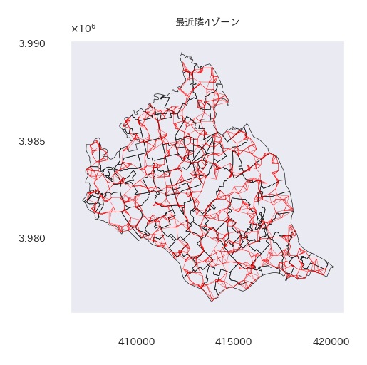
ここで作った隣接行列をこの後にそのまま使うと非対称な隣接行列はダメだってエラーがでた。つまり、地域Aは地域Bと隣接なのに、地域Bは地域Aと隣接ではないという場合があって非対称となってしまっているそうだ。そのため片方が隣接ならもう片方も隣接とするような処理を実施した。(なので地域によっては近隣地域が5以上の場合もあるだろう。)
# 隣接行列作成
adj = wnn2.to_adjlist()
adj_symmetry = np.zeros((len(y_train), len(y_train)))
for i, (focal, neighbor) in tqdm(enumerate(zip(adj['focal'],adj['neighbor']))):
    if (focal, neighbor) in wnn2.asymmetry():
        # 非対称の場合、お互いに1とする
        adj_symmetry[focal, neighbor] = adj_symmetry[neighbor, focal] = 1
        continue
    adj_symmetry[focal, neighbor] = adj_symmetry[neighbor, focal] = 1
print(adj_symmetry.shape)
# >> (851, 851)
土壌分類の数とエンコード済みの土壌分類の配列を定義。
# 土壌分類コードリスト
classK = sorted(y_train[objective_variables].unique())
K = len(classK)
print(classK)
print(K)
# >> [0, 1, 2, 3, 4, 5, 6, 7, 8, 9]
# >> 10
ICARモデル①:空間相関変数は1つのみ
モデルの構築パターンは2つある。
多項ロジスティック回帰の場合、各クラスに空間相関成分を考慮する必要がある。水田の分類の空間相関、建物用地の分類の空間相関、森林の分類の空間相関…など。
これに対応するパターンが2つあり、1つ目が空間相関変数そのものは1つしかないが、その分散がクラスによって異なることでクラスごとに固有の空間相関を表現する方法。2つ目が単純に空間相関変数をクラスの数分用意する方法である。なお今回、うまく収束しない、かつかなり時間がかかるため誤差項は導入せず、回帰係数、切片、空間相関変数のパラメータ推定を実施している。
1つ目のパターンから構築してみる。
以下のコードでは、pm.ICARは1つしか用意していないが、その分散としてtau = pm.Uniform('tau', lower=0, upper=100, dims=("obj_var", ))と定義し次元をクラス数に合わせており、空間相関成分がICARs.reshape((len(y.eval()), 1))*tauによってクラスの数分できるようにしている。
なお、tauをICARsに直接かけ算しているのは、再パラメータ化というテクニックで、MCMCの推論が安定するようにしている。(「ICARモデルのMCMCをPythonで実行する」、「NumPyro:再パラメータ化」)
また、不均衡に対応するためpm.Potentialを使って重み付けも行っている。
with pm.Model() as model:
    # coords(次元やインデックスを定義)
    model.add_coord('data', values=range(X_train.shape[0]), mutable=True)
    model.add_coord('var', values=explanatory_variables, mutable=True)
    model.add_coord('obj_var', values=sorted(y_train[objective_variables].unique()), mutable=True)

    # 変数
    x = pm.MutableData('x', X_train[explanatory_variables].to_numpy(), dims=('data', 'var'))
    y = pm.MutableData("y", y_train[objective_variables].to_numpy(), dims=('data', ))
    weights = pm.MutableData("weights", sample_ws, dims=('data', ))
    # pm_adj_symmetry = pm.MutableData("adj_symmetry", adj_symmetry, dims=('data', 'data'))
    print('x shape', x.eval().shape)
    print('y shape', y.eval().shape)
    print('weights shape', weights.eval().shape)
    # print('pm_adj_symmetry shape', pm_adj_symmetry.eval().shape)
    # 分散
    tau = pm.Uniform('tau', lower=0, upper=100, dims=("obj_var", ))#pm.Exponential('tau', 1)
    print('tau shape', tau.eval().shape)

    # 推論パラメータの事前分布
    coef_ = pm.Normal('coef', mu=0.0, sigma=1, dims=("var",'obj_var'))  # 各係数の事前分布は正規分布
    intercept_ = pm.Normal('intercept', mu=0.0, sigma=1.0, dims=("obj_var", ))  # 切片の事前分布は正規分布
    print('coef shape', coef_.eval().shape)
    print('intercept shape', intercept_.eval().shape)

    # ICAR
    # 空間相関の項は地域の数分あり、クラス別の差異は分散tauで表現
    ICARs = pm.ICAR('z_car', W=adj_symmetry, sigma=1, dims=('data', ))
    print('ICAR type', ICARs.type)
    # linear model
    mu = pm.Deterministic("mu", x.dot(coef_)+intercept_+(ICARs.reshape((len(y.eval()), 1))*tau), dims=('data', 'obj_var'))
    print('x.dot(coef_) shape', x.dot(coef_).eval().shape)
    print('ICARs*tau type', (ICARs*tau).type)
    theta = pm.Deterministic("theta", pm.math.softmax(mu, axis=1), dims=('data', 'obj_var'))  # axis設定しないとダメ
    #y_pred = pm.Categorical("y_pred", p=theta, observed=y, dims='data')
    y_pred = pm.Potential('y_pred', (weights * pm.logp(pm.Categorical.dist(p=theta), y)).sum(axis=0), dims=('data', ))
# モデル構造
modeldag = pm.model_to_graphviz(model)
display(modeldag)

MCMC実行。繰り返し回数は3000、バーンイン期間は1000、チェーンは3つに設定。CPUのみで20分くらいかかった。
%%time
# MCMC実行
# バックエンドでNumPyroで実行
with model:
    # MCMCによる推論
    trace = pm.sample(draws=3000, tune=1000, chains=3, nuts_sampler="numpyro", random_seed=1, return_inferencedata=True, idata_kwargs={"log_likelihood": False})
# >> Wall time: 18min 24s

# 保存
model_dir = '/content/drive/MyDrive/satelite/model'
os.makedirs(model_dir, exist_ok=True)
# データの保存 to_netcdfの利用
trace.to_netcdf(os.path.join(model_dir, 'model_ICAR.nc'))

# Load
model_dir = '/content/drive/MyDrive/satelite/model'
os.makedirs(model_dir, exist_ok=True)
# データの読み込み from_netcdfの利用
trace = az.from_netcdf(os.path.join(model_dir, 'model_ICAR.nc'))
回帰係数と切片のtrace plot。
収束してそうに見える。
# plot_trace
az.plot_trace(trace, backend_kwargs={"constrained_layout":True}, var_names=["coef","intercept"])#+['z_car'+str(i) for i in range(1,11)])
plt.show()

$\hat{R}$で収束の確認。
$\hat{R}$が1.1を超えているか、超えているならそれはどのパラメータかを出力する。全パラメータの$\hat{R}$の最大値は1.67で、複数のパラメータで1.1を超えているのでめちゃくちゃうまく収束しているわけではなさそう。でも1.6とかなのでめちゃくちゃ悪いわけでもない。
%%time
# MCMCの収束を評価
rhat_vals = az.rhat(trace).values()

# 最大のRhatを確認
result = np.max([np.max(i.values) for i in rhat_vals])# if i.name in ["coef","intercept",'z_car','mu','theta','tau']])
print('Max rhat:', result)
# 1.1以上のRhatを確認
for i in rhat_vals:
    if np.max(i.values)>=1.1:
        print(i.name, np.max(i.values), np.mean(i.values), i.values.shape, sep='  ====>  ')

各クラスの事後確率を取り出し、学習データの精度を確認する。
めっちゃ上がったw
# 各クラスの事後確率theta
softmax_result = pd.DataFrame(trace['posterior']['theta'].mean(dim=["chain", "draw"]).values)
y_pred = softmax_result.idxmax(axis=1)
print(sklearn.metrics.classification_report(y_train[objective_variables].to_numpy(), y_pred.ravel()))
cm = sklearn.metrics.confusion_matrix(y_train[objective_variables].to_numpy(), y_pred.ravel())
print(cm)

未知のテストデータへの適用も実施する。
しかしCARモデルで推定した空間相関変数は学習時のデータに対応したものであり、未知のデータの空間相関はわからない。そのため未知のデータに対応するためにはひと工夫必要である。
今回行った工夫は、テストデータの各地域と最も近い学習データの地域を探し出し、その地域の空間相関変数をテストデータに適用するというアプローチ。

k近傍法を使ってテストデータの各サンプルと最も近い学習データのindexを取得する。
# 学習データ、テストデータの座標を取得
train_coord = pd.DataFrame({'x':X_train['geometry'].x.to_list(), 'y':X_train['geometry'].y.to_list()})
test_coord = pd.DataFrame({'x':X_test['geometry'].x.to_list(), 'y':X_test['geometry'].y.to_list()})
# 学習データでknn作成
knn = sklearn.neighbors.NearestNeighbors(n_neighbors=5)
knn.fit(train_coord)
# テストデータの各サンプルと最も近い学習データのindexを取得
distances, indices = knn.kneighbors(test_coord)
test_coord['indices'] = indices[:,0]
display(test_coord)

テストデータの各サンプルと最も近い学習データのindexを使って、テストデータと最も近い学習データの空間相関変数を取得する。
# テストデータと最も近い学習データの空間相関変数を取得する
z_cars_arr = trace['posterior']['z_car'].mean(dim=["chain", "draw"]).values.reshape(-1,1)
z_cars_arr_test = z_cars_arr[list(indices[:,0]),:]  # テストデータと最も近い学習データの空間相関を各テストデータに対して計算
tau_arr = trace['posterior']['tau'].mean(dim=["chain", "draw"]).values
z_cars_arr_test = z_cars_arr_test * tau_arr  # 分散をかける
print(z_cars_arr_test.shape)
# >> (9794, 10)
ベイズ多項ロジスティック回帰の時と同様、推定したパラメータと空間相関変数を使って、線形モデルを定義して推論してあげる必要がある。
F1スコアのマクロ平均を見る感じそこまで良い推論ができているとは言えないが、これまでの空間相関を考慮しないモデルに比べると良い。
# 未知データへの適用
# 回帰係数の推定値
coefs = trace['posterior']['coef'].mean(dim=["chain", "draw"]).values
# 切片の推定値
intercepts = trace['posterior']['intercept'].mean(dim=["chain", "draw"]).values
# 線形モデル式
mu = X_test[explanatory_variables].to_numpy().dot(coefs) + intercepts + z_cars_arr_test  # 回帰式(係数と切片)と空間相関変数
# ソフトマックス関数に入れる
m = softmax(mu, axis=1)  # ソフトマックス関数に入れて一般化線形モデルへ
# 確率が最大のクラスを取得
m_class = m.argmax(axis=1)  # 最も確率が高いクラスを所属クラスとする
# 精度計算
print(sklearn.metrics.classification_report(y_test[objective_variables].to_numpy(), m_class.ravel()))
cm = sklearn.metrics.confusion_matrix(y_test[objective_variables].to_numpy(), m_class.ravel())
print(cm)

推論まで終わったので、実測データ、予測データ、分類成功可否を可視化してみる。
# 実測データ、予測データ、分類成功可否を可視化
def point_plot(results, re_shape_tsukuba_mirai_2RasterCrs, linewidth=0.05, markersize=5, title='', vmin=-8, vmax=8):
    plt.rcParams['font.family'] = prop.get_name() #全体のフォントを設定
    fig = plt.figure(figsize=(9, 3))
    ax = plt.subplot(1,3,1)
    divider = mpl_toolkits.axes_grid1.make_axes_locatable(ax)
    cax = divider.append_axes('right', '5%', pad='3%')
    img = results.plot(column=objective_variables, cmap='tab10', edgecolor='k', legend=True, ax=ax, cax=cax, linewidth=linewidth, markersize=markersize)
    cax.tick_params(labelsize='4', width=0.4, length=5)
    plt.setp(ax.get_xticklabels(), fontsize=4)
    plt.setp(ax.get_yticklabels(), fontsize=4)
    ax.set_title(title+' Point True', fontsize=4)
    re_shape_tsukuba_mirai_2RasterCrs.plot(facecolor='none', edgecolor='k', alpha=0.8, ax=ax, linewidth=0.2)
    ax.yaxis.offsetText.set_fontsize(4)
    ax.yaxis.set_major_formatter(ptick.ScalarFormatter(useMathText=True))
    ax.ticklabel_format(style='sci', axis='y', scilimits=(0,0))
    ax.grid(False)
    cax.set_yticks([c for c in area_use_categories_le.keys()])
    cax.set_yticklabels([c for c in area_use_categories_le.values()])

    ax = plt.subplot(1,3,2)
    divider = mpl_toolkits.axes_grid1.make_axes_locatable(ax)
    cax = divider.append_axes('right', '5%', pad='3%')
    img = results.plot(column='pred', cmap='tab10', edgecolor='k', legend=True, ax=ax, cax=cax, linewidth=linewidth, markersize=markersize)
    cax.tick_params(labelsize='4', width=0.4, length=5)
    plt.setp(ax.get_xticklabels(), fontsize=4)
    plt.setp(ax.get_yticklabels(), fontsize=4)
    ax.set_title(title+' Point Pred', fontsize=4)
    re_shape_tsukuba_mirai_2RasterCrs.plot(facecolor='none', edgecolor='k', alpha=0.8, ax=ax, linewidth=0.2)
    ax.yaxis.offsetText.set_fontsize(4)
    ax.yaxis.set_major_formatter(ptick.ScalarFormatter(useMathText=True))
    ax.ticklabel_format(style='sci', axis='y', scilimits=(0,0))
    ax.grid(False)
    cax.set_yticks([c for c in area_use_categories_le.keys()])
    cax.set_yticklabels([c for c in area_use_categories_le.values()])

    ax = plt.subplot(1,3,3)
    divider = mpl_toolkits.axes_grid1.make_axes_locatable(ax)
    cax = divider.append_axes('right', '5%', pad='3%')
    img = results.plot(column='diff', cmap='binary', edgecolor='k', legend=True, ax=ax, cax=cax, linewidth=linewidth, markersize=markersize, vmin=vmin, vmax=vmax)
    cax.tick_params(labelsize='4', width=0.4, length=5)
    plt.setp(ax.get_xticklabels(), fontsize=4)
    plt.setp(ax.get_yticklabels(), fontsize=4)
    ax.set_title(title+' Point False:1, True:0', fontsize=4)
    re_shape_tsukuba_mirai_2RasterCrs.plot(facecolor='none', edgecolor='k', alpha=0.8, ax=ax, linewidth=0.2)
    ax.yaxis.offsetText.set_fontsize(4)
    ax.yaxis.set_major_formatter(ptick.ScalarFormatter(useMathText=True))
    ax.ticklabel_format(style='sci', axis='y', scilimits=(0,0))
    ax.grid(False)
    plt.tight_layout()
    plt.show()

# 可視化
# 学習データ
results = y_train.copy()
results['pred'] = y_pred.ravel()
results['diff'] = results[objective_variables]-results['pred']
results.loc[(results['diff']==0), 'diff'] = 0
results.loc[(results['diff']!=0), 'diff'] = 1
point_plot(results, re_shape_tsukuba_mirai_2RasterCrs, linewidth=0.05, markersize=5, title='土壌分類', vmin=0, vmax=1)

# テストデータ
results = y_test.copy()
results['pred'] = m_class.ravel()
results['diff'] = results[objective_variables]-results['pred']
results.loc[(results['diff']==0), 'diff'] = 0
results.loc[(results['diff']!=0), 'diff'] = 1
point_plot(results, re_shape_tsukuba_mirai_2RasterCrs, linewidth=0.05, markersize=1, title='土壌分類', vmin=0, vmax=1)
左から、実測、予測、分類成功可否(黒が不正解だった場所)
水田やゴルフ場はまあまあ良さげ。
河川とか建物用地とかが微妙なのかな。
学習データ

テストデータ

ICARモデル②:空間相関変数をクラスの数分定義
2つ目のパターン、単純に空間相関変数をクラスの数分用意する方法を実施する。
以下のコードでは、pm.ICARをクラスの数である10個分用意して空間相関変数10個をICAR10sと定義している。空間相関変数10個の分散は共通したものとしてtau = pm.Uniform('tau', lower=0, upper=100)のようにスカラーとして定義。
tauをICAR10sに直接かけ算して、再パラメータ化している。また、これまでと同様不均衡に対応するためpm.Potentialを使って重み付けも行っている。
with pm.Model() as model:
    # coords(次元やインデックスを定義)
    model.add_coord('data', values=range(X_train.shape[0]), mutable=True)
    model.add_coord('var', values=explanatory_variables, mutable=True)
    model.add_coord('obj_var', values=sorted(y_train[objective_variables].unique()), mutable=True)

    # 変数
    x = pm.MutableData('x', X_train[explanatory_variables].to_numpy(), dims=('data', 'var'))
    y = pm.MutableData("y", y_train[objective_variables].to_numpy(), dims=('data', ))
    weights = pm.MutableData("weights", sample_ws, dims=('data', ))
    print('x shape', x.eval().shape)
    print('y shape', y.eval().shape)
    print('weights shape', weights.eval().shape)

    # 分散
    tau = pm.Uniform('tau', lower=0, upper=100)#pm.Exponential('tau', 1)
    print('tau shape', tau.eval().shape)

    # 推論パラメータの事前分布
    coef_ = pm.Normal('coef', mu=0.0, sigma=1, dims=("var",'obj_var'))  # 各係数の事前分布は正規分布
    intercept_ = pm.Normal('intercept', mu=0.0, sigma=1.0, dims=("obj_var", ))  # 切片の事前分布は正規分布
    print('coef shape', coef_.eval().shape)
    print('intercept shape', intercept_.eval().shape)

    # ICARを10個入ったリストを作ってconcatenateしてdata数×class数の空間相関変数としている
    ICAR10s = [pm.ICAR('z_car'+str(i+1), W=adj_symmetry, sigma=1, dims=('data', )).reshape((len(y.eval()), 1)) for i, k in enumerate(classK)]
    ICAR10s = pm.math.concatenate(ICAR10s, axis=1)

    print('ICAR10s type', ICAR10s.type)
    # linear model --> 𝑦 = coef_𝑥 + intercept_ + eps_ + ICARs
    mu = pm.Deterministic("mu", x.dot(coef_)+intercept_+(ICAR10s*tau), dims=('data', 'obj_var'))
    print('x.dot(coef_) shape', x.dot(coef_).eval().shape)
    print('ICAR10s*tau type', (ICAR10s*tau).type)
    theta = pm.Deterministic("theta", pm.math.softmax(mu, axis=1), dims=('data', 'obj_var'))  # axis設定しないとダメ
    #y_pred = pm.Categorical("y_pred", p=theta, observed=y, dims='data')
    y_pred = pm.Potential('y_pred', (weights * pm.logp(pm.Categorical.dist(p=theta), y)).sum(axis=0), dims=('data', ))

# モデル構造
modeldag = pm.model_to_graphviz(model)
display(modeldag)

MCMC実行。繰り返し回数は3000、バーンイン期間は1000、チェーンは3つに設定。CPUのみで20分くらいかかった。
%%time
# MCMC実行
# バックエンドでNumPyroで実行
with model:
    # MCMCによる推論
    trace = pm.sample(draws=3000, tune=1000, chains=3, nuts_sampler="numpyro", random_seed=1, return_inferencedata=True, idata_kwargs={"log_likelihood": False})

# 保存
model_dir = '/content/drive/MyDrive/satelite/model'
os.makedirs(model_dir, exist_ok=True)
# データの保存 to_netcdfの利用
trace.to_netcdf(os.path.join(model_dir, 'model_ICAR10.nc'))

# Load
model_dir = '/content/drive/MyDrive/satelite/model'
os.makedirs(model_dir, exist_ok=True)
# データの読み込み from_netcdfの利用
trace = az.from_netcdf(os.path.join(model_dir, 'model_ICAR10.nc'))
回帰係数と切片のtrace plot。
収束してそうに見える。
# plot_trace
az.plot_trace(trace, backend_kwargs={"constrained_layout":True}, var_names=["coef","intercept"])#+['z_car'+str(i) for i in range(1,11)])
plt.show()

$\hat{R}$で収束の確認。
$\hat{R}$が1.1を超えているか、超えているならそれはどのパラメータかを出力する。全パラメータの$\hat{R}$の最大値は1.01で、すべて1.1を下回っているのでうまく収束したっぽい。
# MCMCの収束を評価
rhat_vals = az.rhat(trace).values()

# 最大のRhatを確認
result = np.max([np.max(i.values) for i in rhat_vals])# if i.name in ["coef","intercept",'z_car','mu','theta','tau']])
print('Max rhat:', result)
# 1.1以上のRhatを確認
for i in rhat_vals:
    if np.max(i.values)>=1.1:
        print(i.name, np.max(i.values), np.mean(i.values), i.values.shape, sep='  ====>  ')
# >> Max rhat: 1.0112367426367925
>> Max rhat: 1.0112367426367925
各クラスの事後確率を取り出し、学習データの精度を確認する。
前のモデルよりさらに上がったw
# 各クラスの事後確率theta
softmax_result = pd.DataFrame(trace['posterior']['theta'].mean(dim=["chain", "draw"]).values)
y_pred = softmax_result.idxmax(axis=1)
print(sklearn.metrics.classification_report(y_train[objective_variables].to_numpy(), y_pred.ravel()))
cm = sklearn.metrics.confusion_matrix(y_train[objective_variables].to_numpy(), y_pred.ravel())
print(cm)

未知のテストデータへの適用も実施する。
(再掲)k近傍法を使ってテストデータの各サンプルと最も近い学習データのindexを取得する。
# 学習データ、テストデータの座標を取得
train_coord = pd.DataFrame({'x':X_train['geometry'].x.to_list(), 'y':X_train['geometry'].y.to_list()})
test_coord = pd.DataFrame({'x':X_test['geometry'].x.to_list(), 'y':X_test['geometry'].y.to_list()})
# 学習データでknn作成
knn = sklearn.neighbors.NearestNeighbors(n_neighbors=5)
knn.fit(train_coord)
# テストデータの各サンプルと最も近い学習データのindexを取得
distances, indices = knn.kneighbors(test_coord)
test_coord['indices'] = indices[:,0]
display(test_coord)

テストデータの各サンプルと最も近い学習データのindexを使って、テストデータと最も近い学習データの空間相関変数を取得する。
# テストデータと最も近い学習データの空間相関変数を取得する
z_cars_arr = np.concatenate([trace['posterior']['z_car'+str(i+1)].mean(dim=["chain", "draw"]).values.reshape(-1,1) for i, k in enumerate(classK)], axis=1)  # 学習データの空間相関変数の計算
z_cars_arr_test = z_cars_arr[list(indices[:,0]),:]  # テストデータと最も近い学習データの空間相関を各テストデータに対して計算
tau_arr = trace['posterior']['tau'].mean(dim=["chain", "draw"]).values
z_cars_arr_test = z_cars_arr_test * tau_arr  # 分散をかける
print(z_cars_arr_test.shape)
# >> (9794, 10)
これまでと同様、推定したパラメータと空間相関変数を使って、線形モデルを定義して推論する。
F1スコアのマクロ平均を見る感じめちゃくちゃ良い推論ができているとは言えないが、これまでのモデルの中で最も良いし、空間相関を考慮しないモデルより大幅に改善されている。
# 未知データへの適用
# 回帰係数の推定値
coefs = trace['posterior']['coef'].mean(dim=["chain", "draw"]).values
# 切片の推定値
intercepts = trace['posterior']['intercept'].mean(dim=["chain", "draw"]).values
# 線形モデル式
mu = X_test[explanatory_variables].to_numpy().dot(coefs) + intercepts + z_cars_arr_test  # 回帰式(係数と切片)と空間相関変数
# ソフトマックス関数に入れる
m = softmax(mu, axis=1)  # ソフトマックス関数に入れて一般化線形モデルへ
# 確率が最大のクラスを取得
m_class = m.argmax(axis=1)  # 最も確率が高いクラスを所属クラスとする
# 精度計算
print(sklearn.metrics.classification_report(y_test[objective_variables].to_numpy(), m_class.ravel()))
cm = sklearn.metrics.confusion_matrix(y_test[objective_variables].to_numpy(), m_class.ravel())
print(cm)

推論まで終わったので、実測データ、予測データ、分類成功可否データを可視化してみる。
# 可視化
# 学習データ
results = y_train.copy()
results['pred'] = y_pred.ravel()
results['diff'] = results[objective_variables]-results['pred']
results.loc[(results['diff']==0), 'diff'] = 0
results.loc[(results['diff']!=0), 'diff'] = 1
point_plot(results, re_shape_tsukuba_mirai_2RasterCrs, linewidth=0.05, markersize=5, title='土壌分類', vmin=0, vmax=1)

# テストデータ
results = y_test.copy()
results['pred'] = m_class.ravel()
results['diff'] = results[objective_variables]-results['pred']
results.loc[(results['diff']==0), 'diff'] = 0
results.loc[(results['diff']!=0), 'diff'] = 1
point_plot(results, re_shape_tsukuba_mirai_2RasterCrs, linewidth=0.05, markersize=1, title='土壌分類', vmin=0, vmax=1)
左から、実測、予測、分類成功可否(黒が不正解だった場所)
水田、農用地、ゴルフ場はまあまあ良さげ。
南の方の河川の範囲が実際より広いな。
確かにICARモデル①より水田の土地の分類ミスが少ないように見える。それで精度が良くなったのかも。
学習データ

テストデータ

ICARモデル②を使って考察
空間相関を考慮しないベイズロジスティック回帰の回帰係数、切片とICARモデル②の回帰係数、切片、空間相関変数の事後分布をバイオリンプロットで可視化して見てみる。(オッズ比の分析とかはしない…。)
# バイオリンプロット
png_path = '/content/drive/MyDrive/satelite/png/'
os.makedirs(png_path, exist_ok=True)
figsize=(8,6)
plt.rcParams['font.family'] = prop.get_name()
fig=plt.figure(figsize=figsize)
for k, node in enumerate(classK):
    softmax1_org = trace_org['posterior']['coef'].mean(dim=["chain"]).values[:,:,k]
    softmax1 = trace['posterior']['coef'].mean(dim=["chain"]).values[:,:,k]
    corf_df_org = pd.DataFrame(softmax1_org)
    corf_df_org.columns=explanatory_variables
    corf_df_org['intercept'] = trace_org['posterior']['intercept'].mean(dim=["chain"]).values[:,k]
    corf_df_org['tau'] = np.nan
    corf_df_org_stack = corf_df_org.stack().reset_index()
    corf_df_org_stack['space_corr'] = 0
    corf_df_org_stack.columns=['id','col_name','coef','space_corr']
    corf_df = pd.DataFrame(softmax1)
    corf_df.columns=explanatory_variables
    corf_df['intercept'] = trace['posterior']['intercept'].mean(dim=["chain"]).values[:,k]
    corf_df['tau'] = trace['posterior']['tau'].mean(dim=["chain"]).values
    corf_df_stack = corf_df.stack().reset_index()
    corf_df_stack['space_corr'] = 1
    corf_df_stack.columns=['id','col_name','coef','space_corr']
    corf_df_stack = pd.concat([corf_df_org_stack, corf_df_stack]).reset_index(drop=True)

    ax1 = plt.subplot(3,4,k+1)
    img = sns.violinplot(data=corf_df_stack, x='col_name', y='coef', hue="space_corr", split=True, inner="quart", density_norm='width', ax=ax1, linewidth=0.2)
    torf_orgs = {}
    torfs = {}
    for i, col in enumerate(corf_df.columns):
        if col=='tau':
            ax1.text(ax1.get_xticks()[i], corf_df[col].mean(), round(corf_df[col].mean(),2), fontsize=3, ha="left", color="k")
            ax1.text(ax1.get_xticks()[i], corf_df[col].quantile(0.95), round(corf_df[col].quantile(0.95),2), fontsize=2, ha="left", color="k")
            ax1.text(ax1.get_xticks()[i], corf_df[col].quantile(0.05), round(corf_df[col].quantile(0.05),2), fontsize=2, ha="left", color="k")
        else:
            ax1.text(ax1.get_xticks()[i], corf_df_org[col].mean(), round(corf_df_org[col].mean(),2), fontsize=3, ha="right", color="k")
            ax1.text(ax1.get_xticks()[i], corf_df[col].mean(), round(corf_df[col].mean(),2), fontsize=3, ha="left", color="k")

            ax1.text(ax1.get_xticks()[i], corf_df_org[col].quantile(0.95), round(corf_df_org[col].quantile(0.95),2), fontsize=2, ha="right", color="k")
            ax1.text(ax1.get_xticks()[i], corf_df[col].quantile(0.95), round(corf_df[col].quantile(0.95),2), fontsize=2, ha="left", color="k")

            ax1.text(ax1.get_xticks()[i], corf_df_org[col].quantile(0.05), round(corf_df_org[col].quantile(0.05),2), fontsize=2, ha="right", color="k")
            ax1.text(ax1.get_xticks()[i], corf_df[col].quantile(0.05), round(corf_df[col].quantile(0.05),2), fontsize=2, ha="left", color="k")

            if col!='intercept':
                torf_orgs[col] = (corf_df_org[col].quantile(0.95)>=0 and corf_df_org[col].quantile(0.05)<=0)
                torfs[col] = (corf_df[col].quantile(0.95)>=0 and corf_df[col].quantile(0.05)<=0)

    significant_orgs = len([key for key, v in torf_orgs.items() if not v])
    significant = len([key for key, v in torfs.items() if not v])
    ax1.set_xlabel(None)
    ax1.set_ylabel(None)
    plt.setp(ax1.get_xticklabels(), rotation=30, fontsize=4, ha='right')
    plt.setp(ax1.get_yticklabels(), fontsize=4)
    ax1.set_title(f'Class {node}'+' ('+area_use_categories_le[k]+r') coef & $\tau^{2}$, significant:'+str(significant_orgs)+' and '+str(significant), fontsize=4)
    # plt.suptitle(f'Class {node}'+' ('+area_use_categories_le[k]+r') coefficient & $\tau^{2}$', y=0.90, fontsize=4)
    handler, label = ax1.get_legend_handles_labels()
    ax1.legend(handler, ["GLM","ICAR"], fontsize=4, loc='upper left')
plt.tight_layout()
plt.show()
plt.figure().clear()
plt.close()
plt.cla()
plt.clf()
del corf_df_org, corf_df_org_stack, corf_df, corf_df_stack, fig
gc.collect()
水田のクラスの回帰係数を見ると、NDWI(正規化水指数)の回帰係数が大きい。2020年5月2日のデータなので時期的に田んぼに水を張った時期かもしれない。そのためNDWIの影響が大きいのかも。ただICAR②のNDWIの回帰係数の方がベイズ多項ロジスティック回帰より小さくなっている。実際は空間相関の影響が大きいが、回帰係数の影響はそこまで大きくなく、ベイズ多項ロジスティック回帰は回帰係数の影響を過大評価していたのかもしれない。95%信用区間が0を跨ぐ回帰係数の数がベイズ多項ロジスティック回帰よりICAR②の方が多かった。これは水田のクラスだけでなく多くのクラスでも見られた。またどのクラスでも空間相関変数の分散$\tau^{2}$の影響は大きく、実際に推論の精度も上がっていることから、説明変数だけでは説明しきれていない要因が多く空間相関変数によりそれを補っていると思われる。

次に、空間相関変数を面的に図示してみる。
空間相関変数を可視化すると空間パターンが見やすくなる。
# 学習データの空間相関変数を可視化
png_path = '/content/drive/MyDrive/satelite/png/'
os.makedirs(png_path, exist_ok=True)
figsize=(8,6)
plt.rcParams['font.family'] = prop.get_name()
fig=plt.figure(figsize=figsize)
for k, node in enumerate(['z_car'+str(i+1) for i in classK]):
    plot_icar = ground_truth_2RasterCrs_concat_crop_exploded_stats_2point.loc[X_train.index,:].copy()
    icar = trace['posterior'][node].mean(dim=["chain","draw"]).values
    plot_icar[node] = icar
    ax = plt.subplot(3,4,k+1)
    divider = mpl_toolkits.axes_grid1.make_axes_locatable(ax)
    cax = divider.append_axes('right', '5%', pad='3%')
    img = plot_icar.plot(column=node, cmap='RdYlBu_r', edgecolor='k', legend=True, ax=ax, cax=cax, linewidth=0.05, markersize=5)
    cax.tick_params(labelsize='4', width=0.4, length=5)
    plt.setp(ax.get_xticklabels(), fontsize=4)
    plt.setp(ax.get_yticklabels(), fontsize=4)
    ax.set_title(node+' '+area_use_categories_le[k], fontsize=4)
    re_shape_tsukuba_mirai_2RasterCrs.plot(facecolor='none', edgecolor='k', alpha=0.8, ax=ax, linewidth=0.2)
    ax.yaxis.offsetText.set_fontsize(4)
    ax.yaxis.set_major_formatter(ptick.ScalarFormatter(useMathText=True))
    ax.ticklabel_format(style='sci', axis='y', scilimits=(0,0))
    ax.grid(False)
plt.tight_layout()
plt.show()
plt.figure().clear()
plt.close()
plt.cla()
plt.clf()
del plot_icar, fig
gc.collect()

# テストデータの空間相関変数(最も近い学習データの空間相関変数を取得した結果)を可視化
png_path = '/content/drive/MyDrive/satelite/png/'
os.makedirs(png_path, exist_ok=True)
figsize=(8,6)
plt.rcParams['font.family'] = prop.get_name()
fig=plt.figure(figsize=figsize)
for k, node in enumerate(['z_car'+str(i+1) for i in classK]):
    plot_icar = ground_truth_2RasterCrs_concat_crop_exploded_stats_2point.loc[X_test.index,:].copy()
    icar = z_cars_arr_test[:,k]
    plot_icar[node] = icar
    ax = plt.subplot(3,4,k+1)
    divider = mpl_toolkits.axes_grid1.make_axes_locatable(ax)
    cax = divider.append_axes('right', '5%', pad='3%')
    img = plot_icar.plot(column=node, cmap='RdYlBu_r', edgecolor='k', legend=True, ax=ax, cax=cax, linewidth=0.05, markersize=1)
    cax.tick_params(labelsize='4', width=0.4, length=5)
    plt.setp(ax.get_xticklabels(), fontsize=4)
    plt.setp(ax.get_yticklabels(), fontsize=4)
    ax.set_title(node+' '+area_use_categories_le[k], fontsize=4)
    re_shape_tsukuba_mirai_2RasterCrs.plot(facecolor='none', edgecolor='k', alpha=0.8, ax=ax, linewidth=0.2)
    ax.yaxis.offsetText.set_fontsize(4)
    ax.yaxis.set_major_formatter(ptick.ScalarFormatter(useMathText=True))
    ax.ticklabel_format(style='sci', axis='y', scilimits=(0,0))
    ax.grid(False)
plt.tight_layout()
plt.show()
plt.figure().clear()
plt.close()
plt.cla()
plt.clf()
del plot_icar, fig
gc.collect()
各クラス、実際にそのクラスの土壌が分布している地域で空間相関変数の大きさが正の値になっていることが確認できる。例えば水田のクラスを見ると、実際に水田の地域の空間相関変数が正の値になっており、これら地域の推論では水田と分類されやすくなっている。
水田の空間相関変数が大きい地域と被って建物用地の空間相関変数も大きい地域がある。このあたりの地図をGoogle Mapで見てみると確かに水田地帯の中に集落のように住宅街が密集している地域が複数存在している。このあたりの住宅街はもともと田んぼだったところを開発したのかしら。
ゴルフ場の空間パターンを見てみると、森林の空間相関変数が大きい地域と隣接しているように見える。もともと森林地域だったところがゴルフ場になったのかもしれない。
このように連続値としてマッピングすると空間パターンが見やすくなり分析しやすくなる気がする。これがCARモデルを使うメリットだと思う。
学習データ
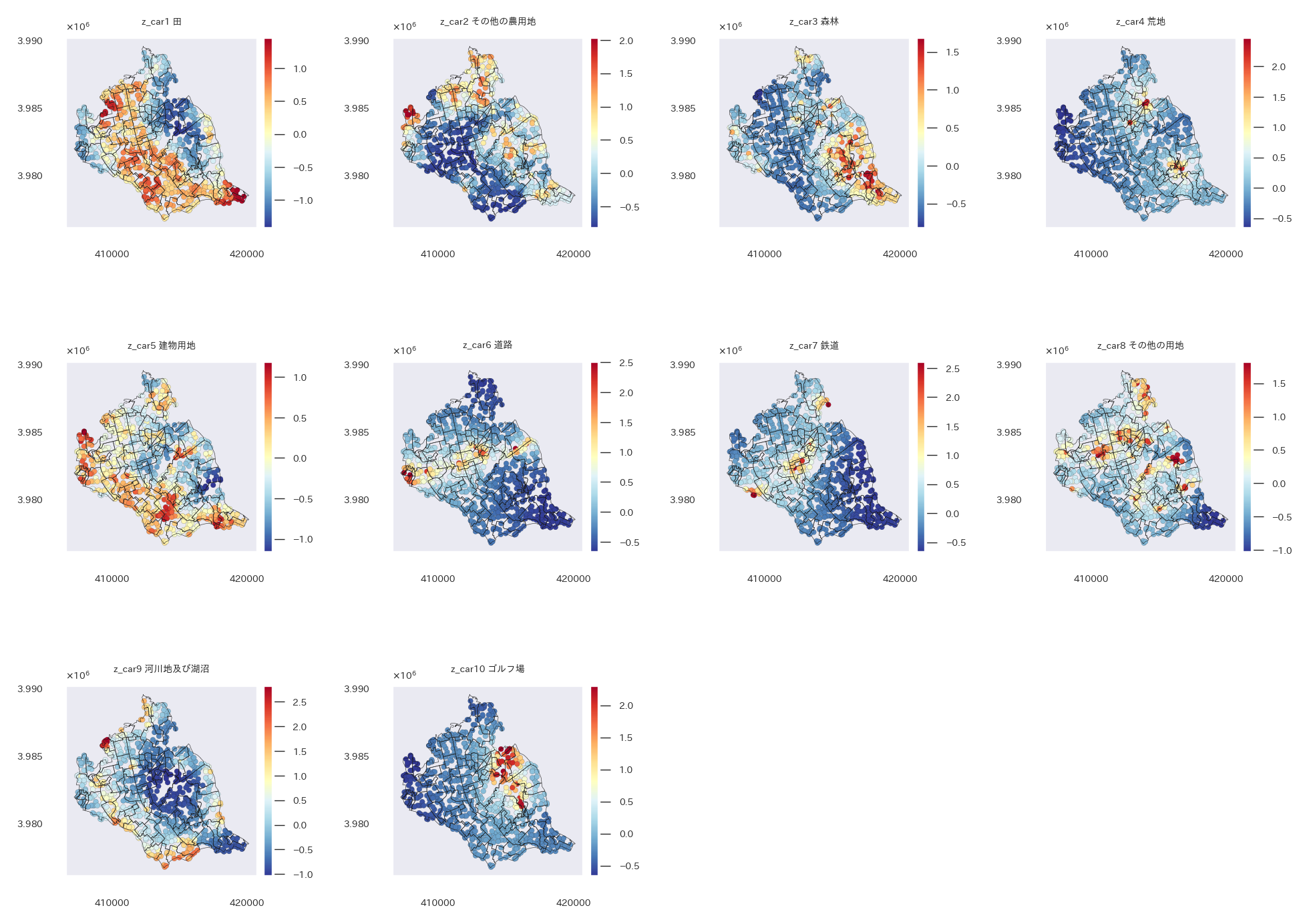
テストデータ

Google Map

4. LightGBM
最後に、空間相関を考慮しないがテーブルデータでは頻出のつよつよモデル、LightGBMでモデリングしてみる。
LightGBM学習。
# LightGBM学習(OptunaのLightGBMTunerCV使用)
params = {'task': 'train',
          'boosting_type': 'gbdt',
          'objective': 'multiclass',
          'metric': 'multi_logloss',
          'verbose': -1,
          'num_class': len(classK),
          'random_state': 0,  # 乱数シード
         }

lgb_train = opt_lgb.Dataset(X_train[explanatory_variables], y_train[objective_variables], weight=sample_ws)
skf = sklearn.model_selection.StratifiedKFold(n_splits=5, shuffle=True, random_state=0)
# LightGBM学習
tuner_cv = opt_lgb.LightGBMTunerCV(params, lgb_train
                                   , num_boost_round=1000
                                   , folds=skf
                                   , return_cvbooster=True
                                   , optuna_seed=0
                                   , callbacks=[opt_lgb.early_stopping(stopping_rounds=50, verbose=True)])

# 最適なパラメータを探索する
tuner_cv.run()
# 最も良かったスコアとパラメータを書き出す
print(f'Best score: {tuner_cv.best_score}')
print('Best params:')
print(tuner_cv.best_params)
推論用関数。
# LightGBMTunerCVでモデル作成時、n_splits数だけモデルができる
# すべてのモデルの結果の平均をとる関数
def cv_model_output(models, X_test):
    preds = []
    for mdl in models:
        pred = mdl.predict(X_test)
        preds.append(pred)
    pred = np.mean(np.array(preds), axis=0)
    return pred
学習データの推論と結果可視化。
# 学習データ推論
models = tuner_cv.get_best_booster()
models = models.boosters
y_pred = cv_model_output(models, X_train[explanatory_variables].to_numpy())
m_class = y_pred.argmax(axis=1)  # 最も確率が高いクラスを所属クラスとする
print(sklearn.metrics.classification_report(y_train[objective_variables].to_numpy(), m_class.ravel()), '\n')
cm = sklearn.metrics.confusion_matrix(y_train[objective_variables].to_numpy(), m_class.ravel())
print(cm, '\n')

# 学習データ推論結果可視化
results = y_train.copy()
results['pred'] = m_class.ravel()
results['diff'] = results[objective_variables]-results['pred']
results.loc[(results['diff']==0), 'diff'] = 0
results.loc[(results['diff']!=0), 'diff'] = 1
point_plot(results, re_shape_tsukuba_mirai_2RasterCrs, linewidth=0.05, markersize=5, title='土壌分類', vmin=0, vmax=1)


テストデータの推論と結果可視化。
# テストデータ推論
y_pred = cv_model_output(models, X_test[explanatory_variables].to_numpy())
m_class = y_pred.argmax(axis=1)  # 最も確率が高いクラスを所属クラスとする
print(sklearn.metrics.classification_report(y_test[objective_variables].to_numpy(), m_class.ravel()), '\n')
cm = sklearn.metrics.confusion_matrix(y_test[objective_variables].to_numpy(), m_class.ravel())
print(cm, '\n')

# テストデータ推論結果可視化
results = y_test.copy()
results['pred'] = m_class.ravel()
results['diff'] = results[objective_variables]-results['pred']
results.loc[(results['diff']==0), 'diff'] = 0
results.loc[(results['diff']!=0), 'diff'] = 1
point_plot(results, re_shape_tsukuba_mirai_2RasterCrs, linewidth=0.05, markersize=1, title='土壌分類', vmin=0, vmax=1)

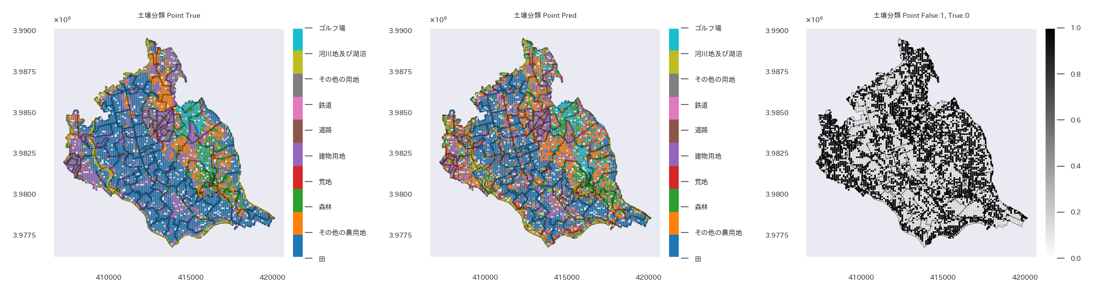
推論精度はICARモデルに負けていた。説明変数だけでは説明しきれていない要因が多いってことがICARモデルの分析からわかっていたので納得。今回は少量サンプルの学習だったので、大量データだったらもう少し良いのかも。ただ、少量データならICARの方が精度もいいし解釈性も高いのでLightGBMを使うメリットはなさそう(学習が早いというメリットはあるが)。
おわりに
土壌分類データで多項分類モデルを以下の4種構築した。
- 多項ロジスティック回帰(ソフトマックス回帰)
- ベイズ多項ロジスティック回帰(ソフトマックス回帰)
- 多項ICARモデル
- LightGBM
ICARモデルが最も良いモデルだった。
いくつかやり残しもあったが(誤差項を入れると収束しない事の解決や、回帰係数がある時の$\frac{\tau^{2}}{\sigma^2+\tau^{2}}$の考え方など)、いろいろ勉強になる取り組みだった。
地理空間データ解析の方法とPyMCによるモデリングが学べたので個人的には満足。
次は時系列も考慮した時空間モデルを試してみたいなぁ。
以上!
追記
この記事で以下のように書いたが、
モデルの構築パターンは2つある。
(中略)
1つ目が空間相関変数そのものは1つしかないが、その分散がクラスによって異なることでクラスごとに固有の空間相関を表現する方法。2つ目が単純に空間相関変数をクラスの数分用意する方法である。
これもう1つパターンがあるなと。パターン1と2の組み合わせを忘れていた。
空間相関変数がクラスの数分あって、かつ分散もクラスの数分あるパターン。
これも一応やってみて、結果を見ておく。
結論を言うと、モデリングの精度自体はパターン2の方が良かった。(パターン1よりはよかった。)
モデル構築。tau = pm.Uniform('tau', lower=0, upper=100, dims=("obj_var", ))のように空間相関変数の分散を10次元で定義。
with pm.Model() as model:
    # coords(次元やインデックスを定義)
    model.add_coord('data', values=range(X_train.shape[0]), mutable=True)
    model.add_coord('var', values=explanatory_variables, mutable=True)
    model.add_coord('obj_var', values=sorted(y_train[objective_variables].unique()), mutable=True)

    # 変数
    x = pm.MutableData('x', X_train[explanatory_variables].to_numpy(), dims=('data', 'var'))
    y = pm.MutableData("y", y_train[objective_variables].to_numpy(), dims=('data', ))
    weights = pm.MutableData("weights", sample_ws, dims=('data', ))
    print('x shape', x.eval().shape)
    print('y shape', y.eval().shape)
    print('weights shape', weights.eval().shape)

    # 分散
    tau = pm.Uniform('tau', lower=0, upper=100, dims=("obj_var", ))
    print('tau shape', tau.eval().shape)

    # 推論パラメータの事前分布
    coef_ = pm.Normal('coef', mu=0.0, sigma=1, dims=("var",'obj_var'))  # 各係数の事前分布は正規分布
    intercept_ = pm.Normal('intercept', mu=0.0, sigma=1.0, dims=("obj_var", ))  # 切片の事前分布は正規分布
    print('coef shape', coef_.eval().shape)
    print('intercept shape', intercept_.eval().shape)

    # ICARを10個入ったリストを作ってconcatenateしてdata数×class数の空間相関変数としている
    ICAR10s = [pm.ICAR('z_car'+str(i+1), W=adj_symmetry, sigma=1, dims=('data', )).reshape((len(y.eval()), 1)) for i, k in enumerate(classK)]
    ICAR10s = pm.math.concatenate(ICAR10s, axis=1)

    print('ICAR10s type', ICAR10s.type)
    # linear model --> 𝑦 = coef_𝑥 + intercept_ + eps_ + ICARs
    mu = pm.Deterministic("mu", x.dot(coef_)+intercept_+(ICAR10s*tau), dims=('data', 'obj_var'))
    print('x.dot(coef_) shape', x.dot(coef_).eval().shape)
    print('ICAR10s*tau type', (ICAR10s*tau).type)
    theta = pm.Deterministic("theta", pm.math.softmax(mu, axis=1), dims=('data', 'obj_var'))  # axis設定しないとダメ
    #y_pred = pm.Categorical("y_pred", p=theta, observed=y, dims='data')
    y_pred = pm.Potential('y_pred', (weights * pm.logp(pm.Categorical.dist(p=theta), y)).sum(axis=0), dims=('data', ))

# モデル構造
modeldag = pm.model_to_graphviz(model)
display(modeldag)

トレースプロットと$\hat{R}$確認。問題なし。
# plot_trace
az.plot_trace(trace, backend_kwargs={"constrained_layout":True}, var_names=["coef","intercept",'tau'])#+['z_car'+str(i) for i in range(1,11)])
plt.show()

# MCMCの収束を評価
rhat_vals = az.rhat(trace).values()

# 最大のRhatを確認
result = np.max([np.max(i.values) for i in rhat_vals])# if i.name in ["coef","intercept",'z_car','mu','theta','tau']])
print('Max rhat:', result)
# 1.1以上のRhatを確認
for i in rhat_vals:
    if np.max(i.values)>=1.1:
        print(i.name, np.max(i.values), np.mean(i.values), i.values.shape, sep='  ====>  ')
# >> Max rhat: 1.0069816457202962

学習データの精度確認。パターン1より良く、パターン2より悪い。
# 各クラスの事後確率theta
softmax_result = pd.DataFrame(trace['posterior']['theta'].mean(dim=["chain", "draw"]).values)
y_pred = softmax_result.idxmax(axis=1)
print(sklearn.metrics.classification_report(y_train[objective_variables].to_numpy(), y_pred.ravel()))
cm = sklearn.metrics.confusion_matrix(y_train[objective_variables].to_numpy(), y_pred.ravel())
print(cm)

テストデータの各サンプルと最も近い学習データのindexを取得するコード。
# 学習データ、テストデータの座標を取得
train_coord = pd.DataFrame({'x':X_train['geometry'].x.to_list(), 'y':X_train['geometry'].y.to_list()})
test_coord = pd.DataFrame({'x':X_test['geometry'].x.to_list(), 'y':X_test['geometry'].y.to_list()})
# 学習データでknn作成
knn = sklearn.neighbors.NearestNeighbors(n_neighbors=5)
knn.fit(train_coord)
# テストデータの各サンプルと最も近い学習データのindexを取得
distances, indices = knn.kneighbors(test_coord)
test_coord['indices'] = indices[:,0]
display(test_coord)

# テストデータと最も近い学習データの空間相関変数を取得する
z_cars_arr = np.concatenate([trace['posterior']['z_car'+str(i+1)].mean(dim=["chain", "draw"]).values.reshape(-1,1) for i, k in enumerate(classK)], axis=1)  # 学習データの空間相関変数の計算
z_cars_arr_test = z_cars_arr[list(indices[:,0]),:]  # テストデータと最も近い学習データの空間相関を各テストデータに対して計算
tau_arr = trace['posterior']['tau'].mean(dim=["chain", "draw"]).values
z_cars_arr_test = z_cars_arr_test * tau_arr  # 分散をかける
print(z_cars_arr_test.shape)
# >> (9794, 10)
テストデータの精度確認。パターン1より良く、パターン2よりやや悪い。
# 未知データへの適用
# 回帰係数の推定値
coefs = trace['posterior']['coef'].mean(dim=["chain", "draw"]).values
# 切片の推定値
intercepts = trace['posterior']['intercept'].mean(dim=["chain", "draw"]).values
# 線形モデル式
mu = X_test[explanatory_variables].to_numpy().dot(coefs) + intercepts + z_cars_arr_test  # 回帰式(係数と切片)と空間相関変数
# ソフトマックス関数に入れる
m = softmax(mu, axis=1)  # ソフトマックス関数に入れて一般化線形モデルへ
# 確率が最大のクラスを取得
m_class = m.argmax(axis=1)  # 最も確率が高いクラスを所属クラスとする
# 精度計算
print(sklearn.metrics.classification_report(y_test[objective_variables].to_numpy(), m_class.ravel()))
cm = sklearn.metrics.confusion_matrix(y_test[objective_variables].to_numpy(), m_class.ravel())
print(cm)
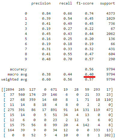
推論結果を可視化。パッと見、パターン2と似ている。北部の建物用地の分類ミスが多いかなぁ。
# 可視化
# 学習データ
results = y_train.copy()
results['pred'] = y_pred.ravel()
results['diff'] = results[objective_variables]-results['pred']
results.loc[(results['diff']==0), 'diff'] = 0
results.loc[(results['diff']!=0), 'diff'] = 1
point_plot(results, re_shape_tsukuba_mirai_2RasterCrs, linewidth=0.05, markersize=5, title='土壌分類', vmin=0, vmax=1)

# テストデータ
results = y_test.copy()
results['pred'] = m_class.ravel()
results['diff'] = results[objective_variables]-results['pred']
results.loc[(results['diff']==0), 'diff'] = 0
results.loc[(results['diff']!=0), 'diff'] = 1
point_plot(results, re_shape_tsukuba_mirai_2RasterCrs, linewidth=0.05, markersize=1, title='土壌分類', vmin=0, vmax=1)


回帰係数と空間相関変数の分散の推定結果のバイオリンプロット。
水田と建物用地の空間相関変数の影響が小さいことがわかる。モデルは、この2つのクラスは説明変数である程度説明できると言っているようだ。
# バイオリンプロット
png_path = 'content/drive/MyDrive/satelite/png/'
os.makedirs(png_path, exist_ok=True)
figsize=(10,6)
plt.rcParams['font.family'] = prop.get_name()
fig=plt.figure(figsize=figsize)
for k, node in enumerate(classK):
    softmax1_org = trace_org['posterior']['coef'].mean(dim=["chain"]).values[:,:,k]
    softmax1 = trace['posterior']['coef'].mean(dim=["chain"]).values[:,:,k]
    corf_df_org = pd.DataFrame(softmax1_org)
    corf_df_org.columns=explanatory_variables
    corf_df_org['intercept'] = trace_org['posterior']['intercept'].mean(dim=["chain"]).values[:,k]
    corf_df_org['tau'] = np.nan
    corf_df_org_stack = corf_df_org.stack().reset_index()
    corf_df_org_stack['space_corr'] = 0
    corf_df_org_stack.columns=['id','col_name','coef','space_corr']
    corf_df = pd.DataFrame(softmax1)
    corf_df.columns=explanatory_variables
    corf_df['intercept'] = trace['posterior']['intercept'].mean(dim=["chain"]).values[:,k]
    corf_df['tau'+str(k)] = trace['posterior']['tau'].mean(dim=["chain"]).values[:,k]
    corf_df_stack = corf_df.stack().reset_index()
    corf_df_stack['space_corr'] = 1
    corf_df_stack.columns=['id','col_name','coef','space_corr']
    corf_df_stack = pd.concat([corf_df_org_stack, corf_df_stack]).reset_index(drop=True)

    ax1 = plt.subplot(3,4,k+1)
    img = sns.violinplot(data=corf_df_stack, x='col_name', y='coef', hue="space_corr", split=True, inner="quart", density_norm='width', ax=ax1, linewidth=0.2)
    torf_orgs = {}
    torfs = {}
    for i, col in enumerate(corf_df.columns):
        if 'tau' in col:
            ax1.text(ax1.get_xticks()[i], corf_df[col].mean(), round(corf_df[col].mean(),2), fontsize=3, ha="left", color="k")
            ax1.text(ax1.get_xticks()[i], corf_df[col].quantile(0.95), round(corf_df[col].quantile(0.95),2), fontsize=2, ha="left", color="k")
            ax1.text(ax1.get_xticks()[i], corf_df[col].quantile(0.05), round(corf_df[col].quantile(0.05),2), fontsize=2, ha="left", color="k")
        else:
            ax1.text(ax1.get_xticks()[i], corf_df_org[col].mean(), round(corf_df_org[col].mean(),2), fontsize=3, ha="right", color="k")
            ax1.text(ax1.get_xticks()[i], corf_df[col].mean(), round(corf_df[col].mean(),2), fontsize=3, ha="left", color="k")

            ax1.text(ax1.get_xticks()[i], corf_df_org[col].quantile(0.95), round(corf_df_org[col].quantile(0.95),2), fontsize=2, ha="right", color="k")
            ax1.text(ax1.get_xticks()[i], corf_df[col].quantile(0.95), round(corf_df[col].quantile(0.95),2), fontsize=2, ha="left", color="k")

            ax1.text(ax1.get_xticks()[i], corf_df_org[col].quantile(0.05), round(corf_df_org[col].quantile(0.05),2), fontsize=2, ha="right", color="k")
            ax1.text(ax1.get_xticks()[i], corf_df[col].quantile(0.05), round(corf_df[col].quantile(0.05),2), fontsize=2, ha="left", color="k")

            if col!='intercept':
                torf_orgs[col] = (corf_df_org[col].quantile(0.95)>=0 and corf_df_org[col].quantile(0.05)<=0)
                torfs[col] = (corf_df[col].quantile(0.95)>=0 and corf_df[col].quantile(0.05)<=0)

    significant_orgs = len([key for key, v in torf_orgs.items() if not v])
    significant = len([key for key, v in torfs.items() if not v])
    ax1.set_xlabel(None)
    ax1.set_ylabel(None)
    plt.setp(ax1.get_xticklabels(), rotation=30, fontsize=4, ha='right')
    plt.setp(ax1.get_yticklabels(), fontsize=4)
    ax1.set_title(f'Class {node}'+' ('+area_use_categories_le[k]+r') coef & $\tau^{2}$, significant:'+str(significant_orgs)+' and '+str(significant), fontsize=4)
    # plt.suptitle(f'Class {node}'+' ('+area_use_categories_le[k]+r') coefficient & $\tau^{2}$', y=0.90, fontsize=4)
    handler, label = ax1.get_legend_handles_labels()
    ax1.legend(handler, ["GLM","ICAR"], fontsize=4, loc='upper left')
plt.tight_layout()
plt.show()
plt.figure().clear()
plt.close()
plt.cla()
plt.clf()
del corf_df_org, corf_df_org_stack, corf_df, corf_df_stack, fig
gc.collect()

学習データとテストデータの空間相関変数を可視化して空間パターンを見る。
空間パターンとしてはパターン2と似ているが、やはり水田と建物用地の空間相関変数の絶対値は小さい。そして他のクラスの空間相関変数の絶対値はパターン2よりも大きくなっている。
パターン2であった、水田の中にも建物用地があるような空間パターンはこのモデルでは見られないようだ。
北部の建物用地の空間パターンも無いので、パターン2の方が納得感はあるかなぁ。
正直こっちのモデルの方が良い結果になるんじゃないかと思ってたが、予想が外れた。原因はよくわかんないや。
# 学習データの空間相関変数を可視化
png_path = 'content/drive/MyDrive/satelite/png/'
os.makedirs(png_path, exist_ok=True)
figsize=(8,6)
plt.rcParams['font.family'] = prop.get_name()
fig=plt.figure(figsize=figsize)
for k, node in enumerate(['z_car'+str(i+1) for i in classK]):
    plot_icar = ground_truth_2RasterCrs_concat_crop_exploded_stats_2point.loc[X_train.index,:].copy()
    icar = trace['posterior'][node].mean(dim=["chain","draw"]).values
    plot_icar[node] = icar
    ax = plt.subplot(3,4,k+1)
    divider = mpl_toolkits.axes_grid1.make_axes_locatable(ax)
    cax = divider.append_axes('right', '5%', pad='3%')
    img = plot_icar.plot(column=node, cmap='RdYlBu_r', edgecolor='k', legend=True, ax=ax, cax=cax, linewidth=0.05, markersize=5)
    cax.tick_params(labelsize='4', width=0.4, length=5)
    plt.setp(ax.get_xticklabels(), fontsize=4)
    plt.setp(ax.get_yticklabels(), fontsize=4)
    ax.set_title(node+' '+area_use_categories_le[k], fontsize=4)
    re_shape_tsukuba_mirai_2RasterCrs.plot(facecolor='none', edgecolor='k', alpha=0.8, ax=ax, linewidth=0.2)
    ax.yaxis.offsetText.set_fontsize(4)
    ax.yaxis.set_major_formatter(ptick.ScalarFormatter(useMathText=True))
    ax.ticklabel_format(style='sci', axis='y', scilimits=(0,0))
    ax.grid(False)
plt.tight_layout()
plt.show()
plt.figure().clear()
plt.close()
plt.cla()
plt.clf()
del plot_icar, fig
gc.collect()

# テストデータの空間相関変数(最も近い学習データの空間相関変数を取得した結果)を可視化
png_path = 'content/drive/MyDrive/satelite/png/'
os.makedirs(png_path, exist_ok=True)
figsize=(8,6)
plt.rcParams['font.family'] = prop.get_name()
fig=plt.figure(figsize=figsize)
for k, node in enumerate(['z_car'+str(i+1) for i in classK]):
    plot_icar = ground_truth_2RasterCrs_concat_crop_exploded_stats_2point.loc[X_test.index,:].copy()
    icar = z_cars_arr_test[:,k]
    plot_icar[node] = icar
    ax = plt.subplot(3,4,k+1)
    divider = mpl_toolkits.axes_grid1.make_axes_locatable(ax)
    cax = divider.append_axes('right', '5%', pad='3%')
    img = plot_icar.plot(column=node, cmap='RdYlBu_r', edgecolor='k', legend=True, ax=ax, cax=cax, linewidth=0.05, markersize=1)
    cax.tick_params(labelsize='4', width=0.4, length=5)
    plt.setp(ax.get_xticklabels(), fontsize=4)
    plt.setp(ax.get_yticklabels(), fontsize=4)
    ax.set_title(node+' '+area_use_categories_le[k], fontsize=4)
    re_shape_tsukuba_mirai_2RasterCrs.plot(facecolor='none', edgecolor='k', alpha=0.8, ax=ax, linewidth=0.2)
    ax.yaxis.offsetText.set_fontsize(4)
    ax.yaxis.set_major_formatter(ptick.ScalarFormatter(useMathText=True))
    ax.ticklabel_format(style='sci', axis='y', scilimits=(0,0))
    ax.grid(False)
plt.tight_layout()
plt.show()
plt.figure().clear()
plt.close()
plt.cla()
plt.clf()
del plot_icar, fig
gc.collect()

