Pythonによる地理空間データのハンドリングまとめ

Last updated at 2025-11-04Posted at 2025-10-28

はじめに

普段、地理空間データを取り扱うことが多いのでよく使う処理をここにまとめることとした。
毎回LLMに聞いて回答待つのも面倒だし。
ラスターデータはrasterio、ベクターデータはgeopandasを使用している。（xarray、rioxarrayとかも使えるようになりたい。）
Pythonだと遅い場合は、GDALのコマンドを直接叩く方法もまとめる。
関数の中に頻繁に書かれているsubprocessによるcpやrmコマンド実行は筆者の環境の都合なので無視していい。

参考

国土数値情報ダウンロードサイト
MODIS公式サイト
Copernicus browser (Sentinel-2 data取得のため)
Geopandas User Guide
Rasterio Advanced Topics
GDAL documentation » Programs
衛星データでつくばみらい市の変化を見てみた（地理空間データ解析）
衛星データでつくばみらい市の土壌分類をしてみた（地理空間データ解析）
その他Perplexity AIが参照したすべてのサイト

import

GDALのインストールとPythonパッケージインストールは済んでいるものとする。

# 必要ライブラリのインポート
# 計算の基本ライブラリ
import numpy as np
import pandas as pd
import matplotlib
import matplotlib.pyplot as plt
import matplotlib.font_manager as fm
import matplotlib.ticker as ptick
import japanize_matplotlib
import seaborn as sns
import mpl_toolkits
from mpl_toolkits.axes_grid1 import make_axes_locatable
import sklearn
from PIL import Image

# 空間データ関連
import xarray as xr
import rioxarray as rxr
import geopandas as gpd
import rasterio as rio
from rasterio import plot
from rasterio.plot import show, plotting_extent
from rasterio.mask import mask
from rasterio.enums import Resampling
from rasterio.features import geometry_mask, shapes
from rasterio.warp import calculate_default_transform, reproject
from rasterio.merge import merge
from rasterio.sample import sample_gen
from geocube.api.core import make_geocube
import shapely
from shapely.geometry import MultiPolygon, Polygon, shape
import osgeo
from osgeo import gdal
from rasterstats import zonal_stats
from exactextract import exact_extract
import jismesh.utils as ju
from geopy.distance import geodesic

# 標準ライブラリ
import os
import zipfile
import glob
import shutil
import itertools
import re
from collections import OrderedDict
import warnings
from tqdm import tqdm
import subprocess

import urllib
from pystac_client import Client
from PIL import Image
import requests
import io

# 日本語フォント読み込み
japanize_matplotlib.japanize()
# jpn_fonts=list(np.sort([ttf for ttf in fm.findSystemFonts() if 'ipaexg' in ttf or 'msgothic' in ttf or 'japan' in ttf or 'ipafont' in ttf]))
# jpn_font=jpn_fonts[0]
jpn_font = japanize_matplotlib.get_font_ttf_path()
prop = fm.FontProperties(fname=jpn_font)
print(jpn_font)
plt.rcParams['font.family'] = prop.get_name() #全体のフォントを設定
# plt.rcParams['figure.dpi'] = 250

pd.options.display.float_format = '{:.5f}'.format
sns.set()

使用データ

国土数値情報のラスターデータ（GeoTIFF）と、ベクターデータ（shp、geojson）をダウンロードして使用。またラスターデータでは衛星データから計算したNDVIも使用。NDVIはSentinel-2のデータから計算してGeoTIFFとして保存した。

ラスターの取り扱い

CRSの変更

EPSG:32654からEPSG:4326に変換する。

とりあえずデータ読み込んでファイルがあることを確認。

# NDVI
NDVI = rio.open(os.path.join(dst_dir, 'NDVI_S2A_54SUE_20230107_0_L2A_B08.tif'))

# 標高3次メッシュ 
dem = gpd.read_file('../data/G04-a-11_5339-jgd_GML/G04-a-11_5339-jgd_ElevationAndSlopeAngleTertiaryMesh.shp')

# 行政区画 東京
tokyo = gpd.read_file('../data/N03-20250101_13_GML/N03-20250101_13.shp')
tokyo = tokyo[~tokyo['N03_004'].isin(['所属未定地', '大島町', '利島村', '新島村', '神津島村', '三宅村', '御蔵島村', '八丈町','青ヶ島村', '小笠原村'])]

# 土地利用細分メッシュ（ラスタ版）データ
landuse = rio.open('../data/L03-b-14_5339/L03-b-14_5339.tif')

rasterio

# ラスターCRSを変換
def rascrs_trans(ras_f, dst_crs='EPSG:4326', save_dir='', mv_dir='', resampling=rio.warp.Resampling.nearest):
    with rio.open(ras_f) as rasd:
        # CRSを3次メッシュデータに合わせる
        src_crs = rasd.crs
        src_transform = rasd.transform
        src_width = rasd.width
        src_height = rasd.height
        src_bounds = rasd.bounds
        # ラスターデータの座標参照系をベクターデータの座標参照系に変換
        transform, width, height = rio.warp.calculate_default_transform(src_crs, dst_crs, src_width, src_height, *src_bounds)
        riometa = rasd.meta.copy()
        riometa.update({'crs': dst_crs,'transform': transform,'width': width,'height': height})

        # 座標参照系を変換したラスターデータを新しいファイルに保存
        with rio.open(os.path.join(save_dir, os.path.basename(rasd.name).split('.tif')[0]+'_toCrs.tif'), 'w', **riometa) as dst:
            for i in range(1, rasd.count + 1):
                rio.warp.reproject(
                    source=rio.band(rasd, i),
                    destination=rio.band(dst, i),
                    src_transform=src_transform,
                    src_crs=src_crs,
                    dst_transform=transform,
                    dst_crs=dst_crs,
                    resampling=resampling
                )
                
    subprocess.run(['cp', os.path.join(save_dir, os.path.basename(rasd.name).split('.tif')[0]+'_toCrs.tif'), mv_dir])
    subprocess.run(['rm', os.path.join(save_dir, os.path.basename(rasd.name).split('.tif')[0]+'_toCrs.tif')])

ras_f = os.path.join(dst_dir, 'NDVI_S2A_54SUE_20230107_0_L2A_B08.tif')
rascrs_trans(ras_f, dst_crs='EPSG:4326', save_dir=temp_dir, mv_dir=dst_dir, resampling=rio.warp.Resampling.nearest)

gdal コマンド

# ラスターCRSを変換
def gdal_rascrs_trans(ras_f, dst_crs='EPSG:4326', save_dir='', mv_dir=''):
    subprocess.run(['gdalwarp', '-t_srs', dst_crs, ras_f, os.path.join(save_dir, os.path.basename(rasd.name).split('.tif')[0]+'_toCrsGdal.tif')])
    subprocess.run(['cp', os.path.join(save_dir, os.path.basename(rasd.name).split('.tif')[0]+'_toCrsGdal.tif'), mv_dir])
    subprocess.run(['rm', os.path.join(save_dir, os.path.basename(rasd.name).split('.tif')[0]+'_toCrsGdal.tif')])

ras_f = os.path.join(dst_dir, 'NDVI_S2A_54SUE_20230107_0_L2A_B08.tif')
gdal_rascrs_trans(ras_f, dst_crs='EPSG:4326', save_dir=temp_dir, mv_dir=dst_dir)

結果可視化

左から、オリジナル、rasterioアプローチ、gdalアプローチ

リサンプリング

解像度を変更する。

とりあえずデータ読み込んでファイルがあることを確認。

# NDVI
rioNDVI = rio.open(os.path.join(dst_dir, 'NDVI_S2A_54SUE_20230107_0_L2A_B08_toCrsGdal.tif'))

# 標高3次メッシュ 
dem = gpd.read_file('../data/G04-a-11_5339-jgd_GML/G04-a-11_5339-jgd_ElevationAndSlopeAngleTertiaryMesh.shp')

# 行政区画 東京
tokyo = gpd.read_file('../data/N03-20250101_13_GML/N03-20250101_13.shp')
tokyo = tokyo[~tokyo['N03_004'].isin(['所属未定地', '大島町', '利島村', '新島村', '神津島村', '三宅村', '御蔵島村', '八丈町','青ヶ島村', '小笠原村'])]

# 土地利用細分メッシュ（ラスタ版）データ
landuse = rio.open('../data/L03-b-14_5339/L03-b-14_5339.tif')

gdalコマンドで手元のデータの解像度（ピクセルサイズ）を知りたい時、以下コマンドでPixel Sizeを見る。

subprocess.run(['gdalinfo', os.path.join(dst_dir, 'NDVI_S2A_54SUE_20230107_0_L2A_B08_toCrsGdal.tif')])
subprocess.run(['gdalinfo', '../data/L03-b-14_5339/L03-b-14_5339.tif'])
'''
<略>
Data axis to CRS axis mapping: 2,1
Origin = (138.777603533479947,36.140701996645092)
Pixel Size = (0.000101123343356,-0.000101123343356)
<略>
'''

rasterioで見る場合は以下。

with rio.open(tif_name) as src:
    pixel_size_x = src.transform.a  # X方向のピクセルサイズ
    pixel_size_y = src.transform.e  # Y方向のピクセルサイズ（絶対値）

rasterio (resampling & crop)

ラスターデータAをラスターデータBの解像度、範囲に合わせる場合。（CRSは一致しているとする。）

# ラスターresampling & crop
def ras_resampling_crop(ras_f, dst_f, save_dir='', mv_dir='', resampling=rio.warp.Resampling.nearest):
    with rio.open(ras_f) as src_a:
        with rio.open(dst_f) as src_b:
            # メタデータを取得
            dst_crs = src_b.crs
            dst_transform = src_b.transform
            dst_height = src_b.height
            dst_width = src_b.width

            # ラスターデータをリサンプリング
            # 出力配列を準備
            dst_array = np.empty((src_a.count, dst_height, dst_width), dtype=src_a.dtypes[0])
            
            # リサンプリング実行
            rio.warp.reproject(
                source=rio.band(src_a, list(range(1, src_a.count + 1))),
                destination=dst_array,
                src_transform=src_a.transform,
                src_crs=src_a.crs,
                dst_transform=dst_transform,
                dst_crs=dst_crs,
                resampling=resampling  # リサンプリング方法を指定
            )
            
            # 新しいメタデータを作成
            out_meta = src_a.meta.copy()
            out_meta.update({
                'crs': dst_crs,
                'transform': dst_transform,
                'width': dst_width,
                'height': dst_height
            })
            
            # 結果を保存
            with rio.open(os.path.join(save_dir, os.path.basename(src_a.name).split('.tif')[0]+'_resampling_crop.tif'), 'w', **out_meta) as dst:
                dst.write(dst_array)

            subprocess.run(['cp', os.path.join(save_dir, os.path.basename(src_a.name).split('.tif')[0]+'_resampling_crop.tif'), mv_dir])
            subprocess.run(['rm', os.path.join(save_dir, os.path.basename(src_a.name).split('.tif')[0]+'_resampling_crop.tif')])

ras_f = os.path.join(dst_dir, 'NDVI_S2A_54SUE_20230107_0_L2A_B08_toCrsGdal.tif')
dst_f = '../data/L03-b-14_5339/L03-b-14_5339.tif'
ras_resampling_crop(ras_f, dst_f, save_dir=temp_dir, mv_dir=dst_dir, resampling=rio.warp.Resampling.bilinear)

rasterio (resampling)

ラスターデータAの解像度をラスターデータBの解像度に合わせる場合。（CRSは一致しているとする。）

# ラスターresampling
def ras_resampling(ras_f, dst_f, save_dir='', mv_dir='', resampling=rio.warp.Resampling.nearest):
    with rio.open(ras_f) as src_a:
        with rio.open(dst_f) as src_b:
            # 解像度の比率を計算
            scale_factor_x = src_a.transform.a / src_b.transform.a
            scale_factor_y = abs(src_a.transform.e / src_b.transform.e)
            
            # リサンプリング
            data = src_a.read(
                out_shape=(
                    src_a.count,
                    int(src_a.height * scale_factor_y),
                    int(src_a.width * scale_factor_x)
                ),
                resampling=resampling
            )
            
            # transformを更新（範囲は同じで解像度だけ変更）
            new_transform = src_a.transform * src_a.transform.scale(
                (src_a.width / data.shape[-1]),
                (src_a.height / data.shape[-2])
            )
            
            # メタデータを更新
            out_meta = src_a.meta.copy()
            out_meta.update({
                'transform': new_transform,
                'width': data.shape[-1],
                'height': data.shape[-2]
            })
            
            # 保存
            with rio.open(os.path.join(save_dir, os.path.basename(src_a.name).split('.tif')[0]+'_resampling.tif'), 'w', **out_meta) as dst:
                dst.write(data)
                
            subprocess.run(['cp', os.path.join(save_dir, os.path.basename(src_a.name).split('.tif')[0]+'_resampling.tif'), mv_dir])
            subprocess.run(['rm', os.path.join(save_dir, os.path.basename(src_a.name).split('.tif')[0]+'_resampling.tif')])

ras_f = os.path.join(dst_dir, 'NDVI_S2A_54SUE_20230107_0_L2A_B08_toCrsGdal.tif')
dst_f = '../data/L03-b-14_5339/L03-b-14_5339.tif'
ras_resampling(ras_f, dst_f, save_dir=temp_dir, mv_dir=dst_dir, resampling=rio.warp.Resampling.bilinear)

gdal コマンド (resampling)

ラスターデータAの解像度をラスターデータBの解像度に合わせる場合。（CRSは一致しているとする。）

def gdal_ras_resampling(ras_f, dst_f, save_dir='', mv_dir='', resampling='bilinear'):
    with rio.open(dst_f) as src:
        pixel_size_x = src.transform.a  # X方向のピクセルサイズ
        pixel_size_y = src.transform.e  # Y方向のピクセルサイズ（絶対値）
        print(f"Pixel size X: {pixel_size_x}, Y: {pixel_size_y}")
    # 解像度を-trで指定
    subprocess.run(['gdalwarp', '-tr', str(pixel_size_x), str(pixel_size_y), '-r', resampling, ras_f, os.path.join(save_dir, os.path.basename(ras_f).split('.tif')[0]+'_resamplingGdal.tif')])
    subprocess.run(['cp', os.path.join(save_dir, os.path.basename(ras_f).split('.tif')[0]+'_resamplingGdal.tif'), mv_dir])
    subprocess.run(['rm', os.path.join(save_dir, os.path.basename(ras_f).split('.tif')[0]+'_resamplingGdal.tif')])

ras_f = os.path.join(dst_dir, 'NDVI_S2A_54SUE_20230107_0_L2A_B08_toCrsGdal.tif')
dst_f = '../data/L03-b-14_5339/L03-b-14_5339.tif'
gdal_ras_resampling(ras_f, dst_f, save_dir=temp_dir, mv_dir=dst_dir, resampling='bilinear')

結果可視化

左上：オリジナル（shape:(9945, 12184)）
右上：rasterio (resampling)（shape:(1206, 985)）
左下：gdal コマンド (resampling)（shape:(1207, 986)）
右下：rasterio (resampling & crop)（shape:(800, 800)）

クロップ

任意の座標範囲に切り取る。

とりあえずデータ読み込んでファイルがあることを確認。行政区画データは島嶼部を除いたものを保存しておく。（GDALコマンドで使用。）

# NDVI
rioNDVI = rio.open(os.path.join(dst_dir, 'NDVI_S2A_54SUE_20230107_0_L2A_B08_toCrsGdal.tif'))

# 標高3次メッシュ 
dem = gpd.read_file('../data/G04-a-11_5339-jgd_GML/G04-a-11_5339-jgd_ElevationAndSlopeAngleTertiaryMesh.shp')

# 行政区画 東京
tokyo = gpd.read_file('../data/N03-20250101_13_GML/N03-20250101_13.shp')
tokyo = tokyo[~tokyo['N03_004'].isin(['所属未定地', '大島町', '利島村', '新島村', '神津島村', '三宅村', '御蔵島村', '八丈町','青ヶ島村', '小笠原村'])]
tokyo.to_crs('EPSG:4326').to_file('../data/N03-20250101_13_GML/N03-20250101_13_ep4326.geojson', driver='GeoJSON')
tokyo = gpd.read_file('../data/N03-20250101_13_GML/N03-20250101_13_ep4326.geojson')

# 土地利用細分メッシュ（ラスタ版）データ
landuse = rio.open('../data/L03-b-14_5339/L03-b-14_5339.tif')

rasterio：ポリゴンの範囲に切り取る

# ポリゴンの範囲に切り取る
def ras_crop(ras_f, gdf, save_dir='', mv_dir=''):
    with rio.open(ras_f) as src:
        # CRSを合わせる（重要！）
        gdf_reprojected = gdf.to_crs(src.crs)
        
        # ジオメトリを取得
        shapes = gdf_reprojected.geometry.values
        
        # マスク処理を実行
        out_image, out_transform = rio.mask.mask(
            src, 
            shapes, 
            crop=True,  # Trueでポリゴンの範囲に切り取る
            all_touched=False,  # Trueでポリゴンに触れるピクセルも含める
            nodata=np.nan  # マスク外の値
        )
        
        # メタデータを更新
        out_meta = src.meta.copy()
        out_meta.update({
            "driver": "GTiff",
            "height": out_image.shape[1],
            "width": out_image.shape[2],
            "transform": out_transform,
            'dtype': 'float32'
        })
        
        # 結果を保存
        with rio.open(os.path.join(save_dir, os.path.basename(ras_f).split('.tif')[0]+'_crop.tif'), 'w', **out_meta) as dst:
            dst.write(out_image)
    
        subprocess.run(['cp', os.path.join(save_dir, os.path.basename(ras_f).split('.tif')[0]+'_crop.tif'), mv_dir])
        subprocess.run(['rm', os.path.join(save_dir, os.path.basename(ras_f).split('.tif')[0]+'_crop.tif')])

ras_f = os.path.join(dst_dir, 'NDVI_S2A_54SUE_20230107_0_L2A_B08_toCrsGdal.tif')
ras_crop(ras_f, tokyo, save_dir=temp_dir, mv_dir=dst_dir)

rasterio：bboxの範囲に切り取る

# bboxの範囲に切り取る
def ras_crop_bbox(ras_f, bbox, save_dir='', mv_dir=''):
    # 矩形ポリゴンを作成
    bbox_polygon = shapely.geometry.box(*bbox)
    with rio.open(ras_f) as src:        
        # マスク処理を実行
        out_image, out_transform = rio.mask.mask(
            src, 
            [bbox_polygon], 
            crop=True,  # Trueでポリゴンの範囲に切り取る
            all_touched=False,  # Trueでポリゴンに触れるピクセルも含める
            nodata=np.nan  # マスク外の値
        )
        
        # メタデータを更新
        out_meta = src.meta.copy()
        out_meta.update({
            "driver": "GTiff",
            "height": out_image.shape[1],
            "width": out_image.shape[2],
            "transform": out_transform,
            'dtype': 'float32'
        })
        
        # 結果を保存
        with rio.open(os.path.join(save_dir, os.path.basename(ras_f).split('.tif')[0]+'_crop_bbox.tif'), 'w', **out_meta) as dst:
            dst.write(out_image)
    
        subprocess.run(['cp', os.path.join(save_dir, os.path.basename(ras_f).split('.tif')[0]+'_crop_bbox.tif'), mv_dir])
        subprocess.run(['rm', os.path.join(save_dir, os.path.basename(ras_f).split('.tif')[0]+'_crop_bbox.tif')])

# 切り取りたい範囲を指定 (xmin, ymin, xmax, ymax)
bbox = (138.94286759-0.05,  35.50125223-0.05, 139.91890837+0.05,  35.898424+0.05)
ras_crop_bbox(ras_f, bbox, save_dir=temp_dir, mv_dir=dst_dir)

gdalコマンド：ポリゴンの範囲に切り取る

def gdal_ras_crop(input_tif, polygon_shp, save_dir='', mv_dir=''):
    """gdalwarpコマンドをsubprocessで実行"""
    # polygon_shpとCRSは一致しているように
    command = [
               'gdalwarp',
               # '-s_srs', 'EPSG:4326',      # ソースCRSを明示的に指定
               # '-t_srs', 'EPSG:4326',      # ターゲットCRSも指定（必要に応じて）
               '-cutline', polygon_shp,
               '-crop_to_cutline',
               '-co', 'COMPRESS=LZW',
               '-co', 'TILED=YES',
               '-ot', 'Float32',        # 浮動小数点型を明示的に指定
               '-dstnodata', 'nan',
               input_tif,
               os.path.join(save_dir, os.path.basename(input_tif).split('.tif')[0]+'_cropGdal.tif')
    ]
    
    # 実行
    subprocess.run(command, capture_output=True, text=True)

    subprocess.run(['cp', os.path.join(save_dir, os.path.basename(input_tif).split('.tif')[0]+'_cropGdal.tif'), mv_dir])
    subprocess.run(['rm', os.path.join(save_dir, os.path.basename(input_tif).split('.tif')[0]+'_cropGdal.tif')])

gdal_ras_crop(ras_f, '../data/N03-20250101_13_GML/N03-20250101_13_ep4326.geojson', save_dir=temp_dir, mv_dir=dst_dir)

gdalコマンド：bboxの範囲に切り取る

def gdal_ras_crop_bbox(input_tif, bbox, save_dir='', mv_dir=''):
    # 座標範囲を指定してトリミング
    subprocess.run(['gdalwarp'
                    , '-te', str(bbox[0]), str(bbox[1]), str(bbox[2]), str(bbox[3])
                    # , '-r', 'cubic'
                    , '-co', 'COMPRESS=LZW'
                    , '-co', 'TILED=YES'
                    , '-ot', 'Float32'        # 浮動小数点型を明示的に指定
                    , '-dstnodata', 'nan'
                    , input_tif
                    , os.path.join(save_dir, os.path.basename(input_tif).split('.tif')[0]+'_crop_bboxGdal.tif')])

    subprocess.run(['cp', os.path.join(save_dir, os.path.basename(input_tif).split('.tif')[0]+'_crop_bboxGdal.tif'), mv_dir])
    subprocess.run(['rm', os.path.join(save_dir, os.path.basename(input_tif).split('.tif')[0]+'_crop_bboxGdal.tif')])

bbox = (138.94286759-0.05,  35.50125223-0.05, 139.91890837+0.05,  35.898424+0.05)
gdal_ras_crop_bbox(ras_f, bbox, save_dir=temp_dir, mv_dir=dst_dir)

結果可視化

左上：rasterio (ポリゴンの範囲に切り取る)
右上：rasterio (bboxの範囲に切り取る)
左下：gdal コマンド (ポリゴンの範囲に切り取る)
右下：gdal コマンド (bboxの範囲に切り取る)

マージ

複数のラスターデータを連結する。

とりあえずデータ読み込んでファイルがあることを確認。ラスターデータはCRSが同じ2つのTIFFファイルを使用する。

# NDVI
rioNDVI = rio.open(os.path.join(dst_dir, 'NDVI_S2A_54SUE_20230107_0_L2A_B08_toCrsGdal.tif'))

# 標高3次メッシュ 
dem = gpd.read_file('../data/G04-a-11_5339-jgd_GML/G04-a-11_5339-jgd_ElevationAndSlopeAngleTertiaryMesh.shp')

# 行政区画 東京
# tokyo = gpd.read_file('../data/N03-20250101_13_GML/N03-20250101_13.shp')
# tokyo = tokyo[~tokyo['N03_004'].isin(['所属未定地', '大島町', '利島村', '新島村', '神津島村', '三宅村', '御蔵島村', '八丈町','青ヶ島村', '小笠原村'])]
# tokyo.to_crs('EPSG:4326').to_file('../data/N03-20250101_13_GML/N03-20250101_13_ep4326.geojson', driver='GeoJSON')
tokyo = gpd.read_file('../data/N03-20250101_13_GML/N03-20250101_13_ep4326.geojson')

# 土地利用細分メッシュ（ラスタ版）データ
landuse1 = rio.open('../data/L03-b-14_5339/L03-b-14_5339.tif')
landuse2 = rio.open('../data/L03-b-14_5340/L03-b-14_5340.tif')

rasterio

def ras_merge(tif_files, nodata=np.nan, save_dir='', mv_dir=''):
    """
    複数のTIFファイルをマージして1つのファイルに保存
    """
    
    # ファイルを開く
    src_files = [rio.open(fp) for fp in tif_files]
    
    try:
        # マージ実行
        mosaic, out_trans = rio.merge.merge(
            src_files,
            nodata=nodata,
            dtype='float32'
        )
        
        # メタデータを更新
        out_meta = src_files[0].meta.copy()
        out_meta.update({
            "driver": "GTiff",
            "height": mosaic.shape[1],
            "width": mosaic.shape[2],
            "transform": out_trans,
            "compress": 'lzw',
            "tiled": True,
            "bigtiff": "yes"
        })
        
        # 結果を保存
        with rio.open(os.path.join(save_dir, os.path.basename(tif_files[0]).split('.tif')[0]+'_merge.tif'), 'w', **out_meta) as dest:
            dest.write(mosaic)
        subprocess.run(['cp', os.path.join(save_dir, os.path.basename(tif_files[0]).split('.tif')[0]+'_merge.tif'), mv_dir])
        subprocess.run(['rm', os.path.join(save_dir, os.path.basename(tif_files[0]).split('.tif')[0]+'_merge.tif')])

        
    except Exception as e:
        print(f"Error during merge: {e}")
        return False
        
    finally:
        # ファイルを閉じる
        for src in src_files:
            src.close()

tif_files = ['../data/L03-b-14_5339/L03-b-14_5339.tif', '../data/L03-b-14_5340/L03-b-14_5340.tif']
ras_merge(tif_files, nodata=np.nan, save_dir=temp_dir, mv_dir=dst_dir)

gdalコマンド

# gdalwarpでTIFをマージ
def gdal_ras_merge(tif_files, save_dir='', mv_dir=''):
    """gdalwarpコマンドをsubprocessで実行"""
    # CRSは一致しているように
    subprocess.run([
        'gdalwarp',
        '-co', 'COMPRESS=LZW',
        '-co', 'TILED=YES',
        '-ot', 'Float32',
        '-dstnodata', 'nan',
        *tif_files,
        os.path.join(save_dir, os.path.basename(tif_files[0]).split('.tif')[0]+'_mergeGdal.tif')
    ])
    subprocess.run(['cp', os.path.join(save_dir, os.path.basename(tif_files[0]).split('.tif')[0]+'_mergeGdal.tif'), mv_dir])
    subprocess.run(['rm', os.path.join(save_dir, os.path.basename(tif_files[0]).split('.tif')[0]+'_mergeGdal.tif')])

tif_files = ['../data/L03-b-14_5339/L03-b-14_5339.tif', '../data/L03-b-14_5340/L03-b-14_5340.tif']
gdal_ras_merge(tif_files, save_dir=temp_dir, mv_dir=dst_dir)

結果可視化

左からrasterioアプローチ、gdalアプローチ

Nodata値変更

ここに書くまでもないが、作業頻度は高いので記載。
Nodata値が0だったり、-9999だったりのときに、float型に変えてNodataをNaNに変えるときがあるときのコード。

def ras_nodata_trans(tif_path, new_nodata, nodata=None, save_dir='', mv_dir=''):
    with rio.open(tif_path) as src:
        # データ読み込み
        data = src.read()
        if nodata is None:
            nodata = src.nodata
        data = np.where(data==nodata, new_nodata, data)
        profile = src.profile.copy()
                
        # プロファイル更新
        profile.update({
            'nodata': new_nodata
        })
        if 'int' in profile['dtype']:
            profile.update({
            'dtype': 'float32'
        })
        
        # 出力ファイル作成
        with rio.open(os.path.join(save_dir, os.path.basename(tif_path).split('.tif')[0]+'_transNodata.tif'), 'w', **profile) as dst:
            dst.write(data)
    
        subprocess.run(['cp', os.path.join(save_dir, os.path.basename(tif_path).split('.tif')[0]+'_transNodata.tif'), mv_dir])
        subprocess.run(['rm', os.path.join(save_dir, os.path.basename(tif_path).split('.tif')[0]+'_transNodata.tif')])

tif_path='../data/L03-b-14_5339/L03-b-14_5339.tif'
ras_nodata_trans(tif_path, np.nan, nodata=0, save_dir=temp_dir, mv_dir=dst_dir)

結果可視化。右側のNodata値がNaNになっている。

指数計算

衛星の指数を計算するコード。MODISをベースに作った関数なので、他の衛星データを使う場合はバンドの番号に注意。

def modis_mod09_indices_calculation(file, save_dir='', mv_dir=''):
    """
    MODIS MOD09製品用の衛星指数計算関数
    
    MOD09バンド構成:
    Band 1: Red (620-670 nm)
    Band 2: NIR (841-876 nm) 
    Band 3: Blue (459-479 nm)
    Band 4: Green (545-565 nm)
    Band 5: SWIR1 (1230-1250 nm)
    Band 6: SWIR2 (1628-1652 nm)
    Band 7: SWIR3 (2105-2155 nm)
    """
    
    # 入力データセットを開く
    with rio.open(file) as tif_f:
        # MOD09製品用バンド読み込み
        B1 = tif_f.read(1).astype(float)  # Red
        B2 = tif_f.read(2).astype(float)  # NIR
        B3 = tif_f.read(3).astype(float)  # Blue
        B4 = tif_f.read(4).astype(float)  # Green
        B5 = tif_f.read(5).astype(float)  # SWIR1
        B6 = tif_f.read(6).astype(float)  # SWIR2
        # B7 = tif_f.read(7).astype(float) if tif_f.count >= 7 else None  # SWIR3（7バンドある場合）
        B1 = np.where(B1<0, np.nan, B1)
        B2 = np.where(B2<0, np.nan, B2)
        B3 = np.where(B3<0, np.nan, B3)
        B4 = np.where(B4<0, np.nan, B4)
        B5 = np.where(B5<0, np.nan, B5)
        B6 = np.where(B6<0, np.nan, B6)
        # if tif_f.count >= 7:
        #     B7 = np.where(B7<0, np.nan, B7)
        
        # 0除算回避のための小さな値
        eps = 1e-10
        
        def safe_divide(numerator, denominator):
            """安全な除算（0除算回避）"""
            return np.divide(numerator, denominator, 
                           out=np.full_like(numerator, np.nan), 
                           where=(np.abs(denominator) > eps))
        
        # === 基本植生指数 ===
        
        # 正規化差植生指数（NDVI）= (NIR - Red) / (NIR + Red)
        NDVI = safe_divide(B2 - B1, B2 + B1)
        
        # 強化植生指数（EVI）= 2.5 * (NIR - Red) / (NIR + 6*Red - 7.5*Blue + 1)
        EVI = 2.5 * safe_divide(B2 - B1, B2 + 6*B1 - 7.5*B3 + 1)
        
        # 比植生指数（RVI）= NIR / Red
        RVI = safe_divide(B2, B1)
        
        # 差植生指数（DVI）= NIR - Red
        DVI = B2 - B1
        
        # 土壌調整植生指数（SAVI）= ((NIR - Red) / (NIR + Red + L)) * (1 + L)
        # L = 0.5（標準値）
        L = 0.5
        SAVI = safe_divide(B2 - B1, B2 + B1 + L) * (1 + L)
        
        # === 水関連指数 ===
        
        # 正規化差水指数（NDWI）= (Green - NIR) / (Green + NIR)
        NDWI = safe_divide(B4 - B2, B4 + B2)
        
        # 修正正規化差水指数（MNDWI）= (Green - SWIR1) / (Green + SWIR1)
        MNDWI = safe_divide(B4 - B5, B4 + B5)
        
        # === その他の有用な指数 ===
        
        # Green NDVI = (NIR - Green) / (NIR + Green)
        GNDVI = safe_divide(B2 - B4, B2 + B4)
        
        # 正規化都市化指数（NDBI）= (SWIR1 - NIR) / (SWIR1 + NIR)
        NDBI = safe_divide(B5 - B2, B5 + B2)
        
        # 裸地指数（BSI）= ((SWIR1 + Red) - (NIR + Blue)) / ((SWIR1 + Red) + (NIR + Blue))
        BSI = safe_divide((B5 + B1) - (B2 + B3), (B5 + B1) + (B2 + B3))
        
        # 修正土壌調整植生指数（MSAVI2）
        MSAVI2 = 0.5 * (2 * (B2 + 1) - np.sqrt((2 * B2 + 1)**2 - 8 * (B2 - B1)))

        # BA = NDBI - NDVI（都市域）
        BA = NDBI - NDVI
        
        # UI = (SWIR2 - NIR) / (SWIR2 + NIR)（都市化指数）
        UI = safe_divide(B6 - B2, B6 + B2)
        
        # DBSI = ((SWIR1 - Green) / (SWIR1 + Green)) - NDVI（乾燥裸地指数）
        DBSI = safe_divide(B5 - B4, B5 + B4) - NDVI
        
        # GCI = NIR/Green - 1（Green Chlorophyll Vegetation Index）
        GCI = safe_divide(B2, B4) - 1
        
        # CVI = (NIR/Green) * (Red/Green)（chlorophyll vegetation index）
        CVI = safe_divide(B2, B4) * safe_divide(B1, B4)
        
        # === バンド値（元の関数に合わせて） ===
        Blue = B3
        Green = B4
        Red = B1
        
        # === メタデータ更新 ===
        out_meta = tif_f.meta.copy()
        out_meta.update({
            "count": 1, 
            "nodata": np.nan, 
            "dtype": rio.dtypes.float64
        })
        
        # === 結果リスト（指数名と同じ順序で整理） ===
        indexS = [
            NDVI.reshape(1, tif_f.shape[0], tif_f.shape[1]),           # 正規化差植生指数
            EVI.reshape(1, tif_f.shape[0], tif_f.shape[1]),            # 強化植生指数
            RVI.reshape(1, tif_f.shape[0], tif_f.shape[1]),            # 比植生指数
            DVI.reshape(1, tif_f.shape[0], tif_f.shape[1]),            # 差植生指数
            SAVI.reshape(1, tif_f.shape[0], tif_f.shape[1]),           # 土壌調整植生指数
            NDWI.reshape(1, tif_f.shape[0], tif_f.shape[1]),           # 正規化差水指数
            MNDWI.reshape(1, tif_f.shape[0], tif_f.shape[1]),          # 修正正規化差水指数
            GNDVI.reshape(1, tif_f.shape[0], tif_f.shape[1]),          # Green正規化差植生指数
            NDBI.reshape(1, tif_f.shape[0], tif_f.shape[1]),           # 正規化都市化指数
            BSI.reshape(1, tif_f.shape[0], tif_f.shape[1]),            # 裸地指数
            MSAVI2.reshape(1, tif_f.shape[0], tif_f.shape[1]),         # 修正土壌調整植生指数
            BA.reshape(1, tif_f.shape[0], tif_f.shape[1]),             # BA = NDBI - NDVI（都市域）
            UI.reshape(1, tif_f.shape[0], tif_f.shape[1]),             # UI = (SWIR2 - NIR) / (SWIR2 + NIR)（都市化指数）
            DBSI.reshape(1, tif_f.shape[0], tif_f.shape[1]),           # DBSI = ((SWIR1 - Green) / (SWIR1 + Green)) - NDVI（乾燥裸地指数）
            GCI.reshape(1, tif_f.shape[0], tif_f.shape[1]),            # GCI = NIR/Green - 1（Green Chlorophyll Vegetation Index）
            CVI.reshape(1, tif_f.shape[0], tif_f.shape[1]),            # CVI = (NIR/Green) * (Red/Green)（chlorophyll vegetation index）
            Red.reshape(1, tif_f.shape[0], tif_f.shape[1]),            # Red バンド
            # B2.reshape(1, tif_f.shape[0], tif_f.shape[1]),             # NIR バンド
            Blue.reshape(1, tif_f.shape[0], tif_f.shape[1]),           # Blue バンド
            Green.reshape(1, tif_f.shape[0], tif_f.shape[1]),          # Green バンド
        ]
        indexSName = [
            'NDVI'
            , 'EVI'
            , 'RVI'
            , 'DVI'
            , 'SAVI'
            , 'NDWI'
            , 'MNDWI'
            , 'GNDVI'
            , 'NDBI'
            , 'BSI'
            , 'MSAVI2'
            , 'BA'
            , 'UI'
            , 'DBSI'
            , 'GCI'
            , 'CVI'
            , 'Red'
            , 'Blue'
            , 'Green'
        ]

        indexS_stack = np.vstack(indexS)

        # メタデータをコピー
        profile = tif_f.meta.copy()
        # 出力プロファイル更新
        profile.update({
            'count': indexS_stack.shape[0],
            'dtype': 'float64',  # DOYは小数点を含む可能性
            'nodata': np.nan
        })

        with rio.open(os.path.join(save_dir, os.path.basename(file).split('.tif')[0]+'_index.tif'), 'w', **profile) as dst:
            # 出力書き込み
            dst.write(indexS_stack)
        
        subprocess.run(['cp', os.path.join(save_dir, os.path.basename(file).split('.tif')[0]+'_index.tif'), mv_dir])
        subprocess.run(['rm', os.path.join(save_dir, os.path.basename(file).split('.tif')[0]+'_index.tif')])
    return profile, indexSName

tif_f = '<File Name>'
profile, indexSName = modis_mod09_indices_calculation(tif_f, save_dir=temp_dir, mv_dir=dst_dir)

ラスターからベクターに変換

ラスターデータをベクターデータに変換する。
とりあえずデータ読み込んでファイルがあることを確認。

# NDVI
rioNDVI = rio.open(os.path.join(dst_dir, 'NDVI_S2A_54SUE_20230107_0_L2A_B08_toCrsGdal.tif'))

# 標高3次メッシュ 
dem = gpd.read_file('../data/G04-a-11_5339-jgd_GML/G04-a-11_5339-jgd_ElevationAndSlopeAngleTertiaryMesh.shp')

# 行政区画 東京
# tokyo = gpd.read_file('../data/N03-20250101_13_GML/N03-20250101_13.shp')
# tokyo = tokyo[~tokyo['N03_004'].isin(['所属未定地', '大島町', '利島村', '新島村', '神津島村', '三宅村', '御蔵島村', '八丈町','青ヶ島村', '小笠原村'])]
# tokyo.to_crs('EPSG:4326').to_file('../data/N03-20250101_13_GML/N03-20250101_13_ep4326.geojson', driver='GeoJSON')
tokyo = gpd.read_file('../data/N03-20250101_13_GML/N03-20250101_13_ep4326.geojson')

# 土地利用細分メッシュ（ラスタ版）データ
landuse1 = rio.open('../data/L03-b-14_5339/L03-b-14_5339.tif')
landuse2 = rio.open('../data/L03-b-14_5340/L03-b-14_5340.tif')

rasterio：rio.features.shapesを使用

ラスターのすべてのピクセルが個別にポリゴン化されないので、もともとのピクセル数とGeoDataframeのレコード数は一致しない。

As highlighted using edgecolor='black', neighboring pixels sharing the same raster value are dissolved into larger polygons. The rasterio.features.shapes function unfortunately does not offer a way to avoid this type of dissolving.
https://py.geocompx.org/05-raster-vector

# raster to vector
def ras2vec(tif_f, nodata=None):
    with rio.open(tif_f) as src:
        image = src.read(1)
        if nodata is None:
            nodata = src.nodata
        mask = image != nodata
        
        # ジェネレーターとして取得
        shapes_gen = rio.features.shapes(image, mask=mask, transform=src.transform)
        
        # リストに変換（必要に応じて）
        pol = list(shapes_gen)
        
        # 各要素はタプル (geometry_dict, value)
        geometries = [shape(geom) for geom, val in pol]
        values = [val for geom, val in pol]
        
        gdf = gpd.GeoDataFrame({
            'value': values,
            'geometry': geometries
        }, crs=src.crs)
    return gdf

nodata=None
tif_f = os.path.join(dst_dir, 'NDVI_S2A_54SUE_20230107_0_L2A_B08_toCrsGdal_resampling_crop.tif')
gdf1 = ras2vec(tif_f, nodata=None)
print(gdf1.shape)
display(gdf1.head())

639979行のデータ。（ラスターのピクセル数は640000）

rasterio：全ピクセルをポリゴン化

ラスターのすべてのピクセルをポリゴン化したい場合のコード。

# raster to vector 2
def ras2vec2(tif_f):
    with rio.open(tif_f) as src:
        # 画像サイズを取得
        height = src.height
        width = src.width
        data = src.read(1)
        # 解像度を取得
        pixel_width = abs(src.transform[0])
        pixel_height = abs(src.transform[4])  # 負の値なので絶対値を取る
        
        # 行列インデックスを作成
        rows, cols = np.meshgrid(np.arange(height), np.arange(width), indexing='ij')
    
        # 各ピクセルの左上角の座標を取得
        xs_ul, ys_ul = src.xy(rows.ravel(), cols.ravel(), offset='ul')
        # ポリゴンを作成（box(minx, miny, maxx, maxy)）
        polygons = [
            shapely.geometry.box(x, y - pixel_height, x + pixel_width, y)
            for x, y in tqdm(zip(xs_ul, ys_ul))
        ]
        
        # ピクセルの中心座標を取得
        xs, ys = src.xy(rows.ravel(), cols.ravel())
        # 座標を配列に変換
        x_coords = np.array(xs)
        y_coords = np.array(ys)
        
        # GeoDataFrameを作成
        gdf = gpd.GeoDataFrame({'value':data.ravel(), 'lat':y_coords
                                , 'lon':x_coords
                                , 'id':range(len(y_coords))}
                               , geometry=polygons
                               , crs=src.crs)
    return gdf

tif_f = os.path.join(dst_dir, 'NDVI_S2A_54SUE_20230107_0_L2A_B08_toCrsGdal_resampling_crop.tif')
gdf2 = ras2vec2(tif_f)
print(gdf2.shape)
display(gdf2.head())

640000行のデータ。

結果可視化

左から、オリジナルラスターデータ、ベクターデータ（rio.features.shapesを使用）、ベクターデータ（全ピクセルをポリゴン化）

円形に切り抜く

任意の位置の半径N km周辺を切り抜く。

データ読み込み。

# NDVI
rioNDVI = rio.open(os.path.join(dst_dir, 'NDVI_S2A_54SUE_20230107_0_L2A_B08_toCrsGdal.tif'))

# 標高3次メッシュ 
dem = gpd.read_file('../data/G04-a-11_5339-jgd_GML/G04-a-11_5339-jgd_ElevationAndSlopeAngleTertiaryMesh.shp')

# 行政区画 東京
# tokyo = gpd.read_file('../data/N03-20250101_13_GML/N03-20250101_13.shp')
# tokyo = tokyo[~tokyo['N03_004'].isin(['所属未定地', '大島町', '利島村', '新島村', '神津島村', '三宅村', '御蔵島村', '八丈町','青ヶ島村', '小笠原村'])]
# tokyo.to_crs('EPSG:4326').to_file('../data/N03-20250101_13_GML/N03-20250101_13_ep4326.geojson', driver='GeoJSON')
tokyo = gpd.read_file('../data/N03-20250101_13_GML/N03-20250101_13_ep4326.geojson')

# 土地利用細分メッシュ（ラスタ版）データ
landuse1 = rio.open('../data/L03-b-14_5339/L03-b-14_5339.tif')
landuse2 = rio.open('../data/L03-b-14_5340/L03-b-14_5340.tif')

本来なら、投影座標系で距離を測って切り取った方がいいが、今回はWGS84地理座標系のEPSG:4326のデータを想定して、投影座標系に変換せず概算の距離で円状に切り抜く。

任意の地点での、緯度経度1度あたりの距離を計算する。geopyのgeodesicを使用するとすぐに計算できる。
任意の地点をcoords_pointというPOINTオブジェクトとして定義しているとすると、以下のコードで計算できる。
東京だとおおよそ、1度あたり経度は90.5km、緯度は（どこでもほとんど同じだが）111.0kmとなる。

# 経度1度あたりの距離
dist1deg = geodesic((coords_point.y, coords_point.x), (coords_point.y, coords_point.x+1)).meters
# 緯度1度あたりの距離
dist1deg_lat = geodesic((coords_point.y, coords_point.x), (coords_point.y+1, coords_point.x)).meters

この計算をベースにコードを組む。

def raster_crop_radius4326(raster_path, coords_point, radius_km=10, save_dir='', mv_dir=''):
    # EPSG:4326での距離計算のため度をメートルに変換
    # 概算
    dist1deg = geodesic((coords_point.y, coords_point.x), (coords_point.y, coords_point.x+1)).meters
    dist1deg_lat = geodesic((coords_point.y, coords_point.x), (coords_point.y+1, coords_point.x)).meters
    print(f'経度1度あたりの距離概算{dist1deg} [m]')
    print(f'緯度1度あたりの距離概算{dist1deg_lat} [m]')
    radius_deg = (radius_km*1000)/dist1deg  # 概算での度単位変換
    radius_deg_lat = (radius_km*1000)/dist1deg_lat  # 概算での度単位変換
    print(f'距離{radius_km}kmに該当するdegree', '経度:', radius_deg, '緯度:', radius_deg_lat)

    # 緯度と経度で1度当たりの距離は異なるので処理をはさむ
    # affine変換でX方向とY方向に異なるスケールを適用して楕円に
    # x方向1として、y方向の縮尺
    xfact = 1
    yfact = radius_deg_lat/radius_deg

    # ポイント周辺円状のベクター
    buffered = gpd.GeoDataFrame(geometry=[coords_point], crs="EPSG:4326")
    buffered = buffered.buffer(radius_deg)
    # affine変換でX方向とY方向に異なるスケールを適用して楕円に
    buffered = buffered.geometry.map(lambda geom: shapely.affinity.scale(
        geom, 
        xfact=xfact,  # X方向のスケール
        yfact=yfact   # Y方向のスケール
    ))

    # 切り抜くラスター
    with rio.open(raster_path) as src:
        out_image, out_transform = rio.mask.mask(src, buffered.geometry, crop=True)
        out_meta = src.meta.copy()
    
        # メタデータを更新
        out_meta.update({
            "driver": "GTiff",
            "height": out_image.shape[1],
            "width": out_image.shape[2],
            "transform": out_transform
        })
        # 結果を保存
        output_geotiff = os.path.basename(raster_path).split('.tif')[0]+'_'+str(round(coords_point.x,4))+'_'+str(round(coords_point.y,4))+'.tif'
        with rio.open(os.path.join(save_dir, output_geotiff), "w", **out_meta) as dest:
            dest.write(out_image)
        subprocess.run(['cp', os.path.join(save_dir, output_geotiff), mv_dir])
        subprocess.run(['rm', os.path.join(save_dir, output_geotiff)])

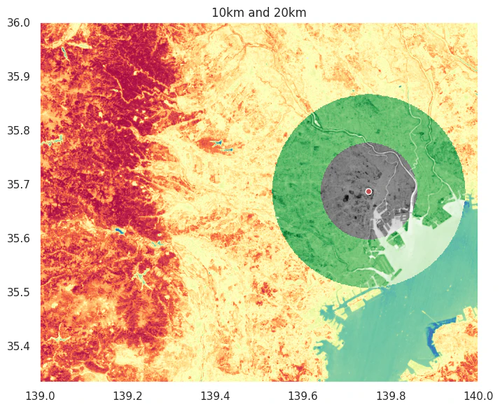
東京のとある市町村区の代表点の周囲10kmと20kmを切り抜く。
結果可視化。

# ベクターgeometry
coords = tokyo.geometry.representative_point().to_numpy()
# 東京のとある市町村区の代表点
coords_point = coords[0]
raster_path = os.path.join(dst_dir, 'NDVI_S2A_54SUE_20230107_0_L2A_B08_toCrsGdal_resampling_crop.tif')
# 10kmで切り抜く
raster_crop_radius4326(raster_path, coords_point, radius_km=10, save_dir=temp_dir, mv_dir=dst_dir)
# >> 経度1度あたりの距離概算90517.95070298456 [m]
# >> 緯度1度あたりの距離概算110962.48443561903 [m]
# >> 距離10kmに該当するdegree 経度: 0.11047532475423441 緯度: 0.09012054885813275

tif_f = os.path.join(mv_dir, output_geotiff)
fig = plt.figure(figsize=(8, 6))
ax = plt.subplot(1,1,1)

# 元のTIF
show(rio.open(os.path.join(dst_dir, 'NDVI_S2A_54SUE_20230107_0_L2A_B08_toCrsGdal_resampling_crop.tif')), ax=ax, cmap='Spectral_r', zorder=1)

# 10kmで切り抜いたTIF
show(rio.open(tif_f), ax=ax, cmap='binary', zorder=3)

# 20kmで切り抜く
raster_crop_radius4326(raster_path, coords_point, radius_km=20, save_dir=temp_dir, mv_dir=dst_dir)
# >> 経度1度あたりの距離概算90517.95070298456 [m]
# >> 緯度1度あたりの距離概算110962.48443561903 [m]
# >> 距離20kmに該当するdegree 経度: 0.22095064950846882 緯度: 0.1802410977162655

tif_f = os.path.join(mv_dir, output_geotiff)
# 20kmで切り抜いたTIF
show(rio.open(tif_f), ax=ax, cmap='Greens', zorder=2)
gpd.GeoDataFrame(geometry=[coords_point], crs="EPSG:4326").plot(ax=ax, color='r', edgecolor='w', markersize=6**2, zorder=4)
ax.set_title('10km and 20km')

plt.tight_layout()
plt.show()

ベクターの取り扱い

CRSの変更

データの読み込み。

# NDVI
rioNDVI = rio.open(os.path.join(dst_dir, 'NDVI_S2A_54SUE_20230107_0_L2A_B08_toCrsGdal.tif'))

# 標高3次メッシュ 
dem = gpd.read_file('../data/G04-a-11_5339-jgd_GML/G04-a-11_5339-jgd_ElevationAndSlopeAngleTertiaryMesh.shp')

# 行政区画 東京
# tokyo = gpd.read_file('../data/N03-20250101_13_GML/N03-20250101_13.shp')
# tokyo = tokyo[~tokyo['N03_004'].isin(['所属未定地', '大島町', '利島村', '新島村', '神津島村', '三宅村', '御蔵島村', '八丈町','青ヶ島村', '小笠原村'])]
# tokyo.to_crs('EPSG:4326').to_file('../data/N03-20250101_13_GML/N03-20250101_13_ep4326.geojson', driver='GeoJSON')
tokyo = gpd.read_file('../data/N03-20250101_13_GML/N03-20250101_13_ep4326.geojson')

# 土地利用細分メッシュ（ラスタ版）データ
landuse1 = rio.open('../data/L03-b-14_5339/L03-b-14_5339.tif')
landuse2 = rio.open('../data/L03-b-14_5340/L03-b-14_5340.tif')

CRSが未定義の場合、set_crsを使う。変更するときはto_crsを使う。

# CRSのセット
# JGD2000: 日本測地系2000
dem4612 = dem.set_crs('EPSG:4612')
# CRSの変更
# WGS84
dem4326 = dem4612.to_crs('EPSG:4326')

結果可視化。

クロップ

データの読み込み。

# NDVI
rioNDVI = rio.open(os.path.join(dst_dir, 'NDVI_S2A_54SUE_20230107_0_L2A_B08_toCrsGdal.tif'))

# 標高3次メッシュ 
dem = gpd.read_file('../data/G04-a-11_5339-jgd_GML/G04-a-11_5339-jgd_ElevationAndSlopeAngleTertiaryMesh.shp')

# 行政区画 東京
# tokyo = gpd.read_file('../data/N03-20250101_13_GML/N03-20250101_13.shp')
# tokyo = tokyo[~tokyo['N03_004'].isin(['所属未定地', '大島町', '利島村', '新島村', '神津島村', '三宅村', '御蔵島村', '八丈町','青ヶ島村', '小笠原村'])]
# tokyo.to_crs('EPSG:4326').to_file('../data/N03-20250101_13_GML/N03-20250101_13_ep4326.geojson', driver='GeoJSON')
tokyo = gpd.read_file('../data/N03-20250101_13_GML/N03-20250101_13_ep4326.geojson')

# 土地利用細分メッシュ（ラスタ版）データ
landuse1 = rio.open('../data/L03-b-14_5339/L03-b-14_5339.tif')
landuse2 = rio.open('../data/L03-b-14_5340/L03-b-14_5340.tif')

# CRSのセット
# JGD2000: 日本測地系2000
dem4612 = dem.set_crs('EPSG:4612')
# CRSの変更
# WGS84
dem4326 = dem4612.to_crs('EPSG:4326')

ベクターデータが2つあり、2つが重複する部分のポリゴンを取得したい時、overlayかsjoinで可能。

# CRSは一致
# 互いに重なっている場所を抽出
dem4326Tokyo = dem4326[['G04a_002', 'geometry']].overlay(tokyo, how='intersection')

# 互いに重なっている場所を抽出
# sjoinでも可能。こっちの方が速い気がする。
# エッジの取り方がoverlayと異なる
dem4326Tokyo = dem4326[['G04a_002', 'geometry']].sjoin(tokyo, how='inner')

結果可視化。左がoverlayで右がsjoin。overlayは重複しない部分のポリゴンは削られて元のポリゴンの形も少し変わるが、sjoinは重複するポリゴンの元の形をそのまま残す。東京都のエッジ部分を見ると分かりやすい。

ベクターデータが2つあり、2つが重複しない部分のポリゴンを取得したい時、overlayのhow='symmetric_difference'で可能。

# 互いに重なっていない場所を抽出
dem4326Tokyo = dem4326[['G04a_002', 'geometry']].overlay(tokyo, how='symmetric_difference')

任意のbboxでクロップしたい時は、GeoDataframeを作ってoverlayやsjoinをする。

# bbox
bbox = (138.94286759-0.01,  35.50125223-0.01, 139.91890837+0.01,  35.898424+0.01)
bbox_polygon = shapely.geometry.box(*bbox)
bboxdf = gpd.GeoDataFrame(geometry=[bbox_polygon], crs=dem4326.crs)
# 互いに重なっている場所を抽出
dem4326Tokyo = dem4326[['G04a_002', 'geometry']].overlay(bboxdf, how='intersection')

ベクターからラスターに変換

データ読み込み。

# NDVI
rioNDVI = rio.open(os.path.join(dst_dir, 'NDVI_S2A_54SUE_20230107_0_L2A_B08_toCrsGdal.tif'))

# 標高3次メッシュ 
dem = gpd.read_file('../data/G04-a-11_5339-jgd_GML/G04-a-11_5339-jgd_ElevationAndSlopeAngleTertiaryMesh.shp')

# 行政区画 東京
# tokyo = gpd.read_file('../data/N03-20250101_13_GML/N03-20250101_13.shp')
# tokyo = tokyo[~tokyo['N03_004'].isin(['所属未定地', '大島町', '利島村', '新島村', '神津島村', '三宅村', '御蔵島村', '八丈町','青ヶ島村', '小笠原村'])]
# tokyo.to_crs('EPSG:4326').to_file('../data/N03-20250101_13_GML/N03-20250101_13_ep4326.geojson', driver='GeoJSON')
tokyo = gpd.read_file('../data/N03-20250101_13_GML/N03-20250101_13_ep4326.geojson')

# 土地利用細分メッシュ（ラスタ版）データ
landuse1 = rio.open('../data/L03-b-14_5339/L03-b-14_5339.tif')
landuse2 = rio.open('../data/L03-b-14_5340/L03-b-14_5340.tif')

# CRSのセット
# JGD2000: 日本測地系2000
dem4612 = dem.set_crs('EPSG:4612')
# CRSの変更
# WGS84
dem4326 = dem4612.to_crs('EPSG:4326')

3次メッシュのベクターを複数の解像度のラスターデータに変換する。
まず3次メッシュのラスターデータのピクセルサイズは事前に確認しておく。
※3次メッシュのピクセルサイズは横0.00125, 縦-0.000833333333である。

# 3次メッシュピクセルサイズ
pixel_width = abs(landuse1.transform[0])
pixel_height = landuse1.transform[4]
print(pixel_width, pixel_height)
# >> 0.00125 -0.000833333333

東京都の範囲にクロップしておく。

# 互いに重なっている場所を抽出
dem4326Tokyo = dem4326[['G04a_002', 'geometry']].sjoin(tokyo, how='inner')
# 数値の型に変換
dem4326Tokyo['G04a_002'] = pd.to_numeric(dem4326Tokyo['G04a_002'], errors='coerce')

ラスター化する。3次メッシュと、より粗い解像度と細かい解像度のラスターデータに変換。

def vec2ras(gdf, colname, pixel_height, pixel_width, fill=np.nan, fname='tmp.tif', save_dir='', mv_dir=''):
    print('ラスター化実行')
    # ラスター化実行
    raster = make_geocube(
        vector_data=gdf[[colname, 'geometry']],
        measurements=[colname],  # 使用する値のカラム
        resolution=(pixel_height, pixel_width),  # ピクセルサイズ
        fill=fill  # 背景値
    )
    print('GeoTIFFとして保存')
    # GeoTIFFとして保存
    output_path = os.path.join(save_dir, fname)
    raster.rio.to_raster(output_path)
    subprocess.run(['cp', output_path, mv_dir])
    subprocess.run(['rm', output_path])

# 3次メッシュ
vec2ras(dem4326Tokyo, 'G04a_002', pixel_height, pixel_width, fill=np.nan
        , fname='dem4326Tokyo.tif', save_dir=temp_dir, mv_dir=dst_dir)
# 低解像度
vec2ras(dem4326Tokyo, 'G04a_002', pixel_height*30, pixel_width*30, fill=np.nan
        , fname='dem4326Tokyo_LowReso.tif', save_dir=temp_dir, mv_dir=dst_dir)
# 高解像度
vec2ras(dem4326Tokyo, 'G04a_002', pixel_height/9, pixel_width/9, fill=np.nan
        , fname='dem4326Tokyo_HighReso.tif', save_dir=temp_dir, mv_dir=dst_dir)

結果可視化。
左上：オリジナルベクターデータ
右上：3次メッシュラスター化
左下：高解像度ラスター化
右下：低解像度ラスター化

ポリゴン内のラスター値の統計量（ゾーン統計）

データ読み込み。

# NDVI
rioNDVI = rio.open(os.path.join(dst_dir, 'NDVI_S2A_54SUE_20230107_0_L2A_B08_toCrsGdal.tif'))

# 標高3次メッシュ 
dem = gpd.read_file('../data/G04-a-11_5339-jgd_GML/G04-a-11_5339-jgd_ElevationAndSlopeAngleTertiaryMesh.shp')

# 行政区画 東京
# tokyo = gpd.read_file('../data/N03-20250101_13_GML/N03-20250101_13.shp')
# tokyo = tokyo[~tokyo['N03_004'].isin(['所属未定地', '大島町', '利島村', '新島村', '神津島村', '三宅村', '御蔵島村', '八丈町','青ヶ島村', '小笠原村'])]
# tokyo.to_crs('EPSG:4326').to_file('../data/N03-20250101_13_GML/N03-20250101_13_ep4326.geojson', driver='GeoJSON')
tokyo = gpd.read_file('../data/N03-20250101_13_GML/N03-20250101_13_ep4326.geojson')

# 土地利用細分メッシュ（ラスタ版）データ
landuse1 = rio.open('../data/L03-b-14_5339/L03-b-14_5339.tif')
landuse2 = rio.open('../data/L03-b-14_5340/L03-b-14_5340.tif')

# CRSのセット
# JGD2000: 日本測地系2000
dem4612 = dem.set_crs('EPSG:4612')
# CRSの変更
# WGS84
dem4326 = dem4612.to_crs('EPSG:4326')
# dem4326.to_file('../data/G04-a-11_5339-jgd_GML/G04-a-11_5339-jgd_ElevationAndSlopeAngleTertiaryMesh_ep4326.geojson', driver='GeoJSON')

rasterstats.zonal_statsを使用

ベクターデータのポリゴン内のラスター値の平均、合計を計算。

# rasterstatsはインストール必要
# ゾーン統計を計算
stats = zonal_stats(
    tokyo.geometry,
    os.path.join(dst_dir, 'NDVI_S2A_54SUE_20230107_0_L2A_B08_toCrsGdal.tif'),
    stats=['mean', 'sum'],
    all_touched=False  # ポリゴンに触れているすべてのピクセルを含めない。ピクセル中心のみ。
)
display(stats)

exactextract.exact_extractを使用

こちらの方がrasterstats.zonal_statsよりも良いらしい。速いし。

# exactextractはインストール必要
# ゾーン統計を計算
# 各ピクセルがポリゴンに覆われている割合（0〜1）を計算し、重み付き平均を算出
stats2 = exact_extract(os.path.join(dst_dir, 'NDVI_S2A_54SUE_20230107_0_L2A_B08_toCrsGdal.tif')
                       , '../data/N03-20250101_13_GML/N03-20250101_13_ep4326.geojson'
                       , ['mean', 'sum'], output='pandas')
display(stats2)

2つのアプローチの比較

結果はおおよそ一致するが、平均値は差異がある。
結果が異なる理由は、AIに聞くとポリゴンに覆われている割合を考慮するかしないかの違いとのこと。

rasterstats（all_touched=Trueの場合）: ポリゴンに触れているピクセルをすべて含め、各ピクセルに重み1を割り当てて単純平均
rasterstats（all_touched=Falseの場合）: ピクセル中心がポリゴン内にあるもののみ含め、各ピクセルに重み1を割り当てて単純平均
exactextract : 各ピクセルがポリゴンに覆われている割合（0〜1）を計算し、重み付き平均を算出

結果可視化

3次メッシュNDVI値から計算した各市町村区の平均値。

ポイントデータの位置に対応するラスター値を取得

ベクターデータのポイントの位置に対応するラスター値を取得する。
この処理は、例えば地上のポイント観測データを所持していて位置に対応した他の変数を作りたい時に活用できる。各地点のNDVIだったり、気温や降水量だったり、標高だったり…。

データの読み込み。

# NDVI
rioNDVI = rio.open(os.path.join(dst_dir, 'NDVI_S2A_54SUE_20230107_0_L2A_B08_toCrsGdal.tif'))

# 標高3次メッシュ 
dem = gpd.read_file('../data/G04-a-11_5339-jgd_GML/G04-a-11_5339-jgd_ElevationAndSlopeAngleTertiaryMesh.shp')

# 行政区画 東京
# tokyo = gpd.read_file('../data/N03-20250101_13_GML/N03-20250101_13.shp')
# tokyo = tokyo[~tokyo['N03_004'].isin(['所属未定地', '大島町', '利島村', '新島村', '神津島村', '三宅村', '御蔵島村', '八丈町','青ヶ島村', '小笠原村'])]
# tokyo.to_crs('EPSG:4326').to_file('../data/N03-20250101_13_GML/N03-20250101_13_ep4326.geojson', driver='GeoJSON')
tokyo = gpd.read_file('../data/N03-20250101_13_GML/N03-20250101_13_ep4326.geojson')

# 土地利用細分メッシュ（ラスタ版）データ
landuse1 = rio.open('../data/L03-b-14_5339/L03-b-14_5339.tif')
landuse2 = rio.open('../data/L03-b-14_5340/L03-b-14_5340.tif')

# CRSのセット
# JGD2000: 日本測地系2000
dem4612 = dem.set_crs('EPSG:4612')
# CRSの変更
# WGS84
dem4326 = dem4612.to_crs('EPSG:4326')
dem4326['G04a_002'] = pd.to_numeric(dem4326['G04a_002'], errors='coerce')

3次メッシュポリゴンの代表位置を取得。

# 3次メッシュポリゴンデータ
data = dem4326[['G04a_002', 'geometry']].copy()
# ポリゴンの代表点をListに格納
coords = [(point.x, point.y) for point in data.geometry.representative_point()]

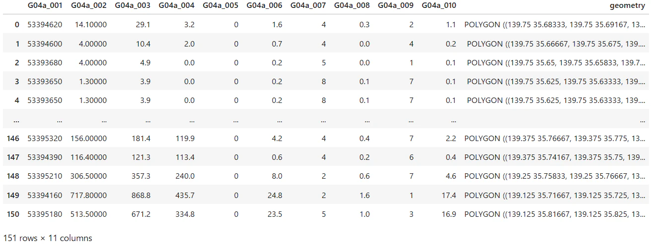
sample_genを使って、各ポイントに対応するラスター値を取得する。

tif_f = os.path.join(dst_dir, 'NDVI_S2A_54SUE_20230107_0_L2A_B08_toCrsGdal.tif')

column_name = os.path.basename(tif_f).split('_')[0]
print(column_name)

with rio.open(tif_f) as src:
    # 値を抽出
    riovalues = np.array(list(sample_gen(src, coords)))
    
extracted_values = riovalues[:,0]
tmp = pd.DataFrame({column_name:extracted_values})
data.loc[:, column_name] = tmp[column_name]
display(data)

結果可視化。3次メッシュのポリゴンのゾーン統計も計算して可視化する。

# ゾーン統計を計算
# 各ピクセルがポリゴンに覆われている割合（0〜1）を計算し、重み付き平均を算出
NDVI_stats = exact_extract(os.path.join(dst_dir, 'NDVI_S2A_54SUE_20230107_0_L2A_B08_toCrsGdal.tif')
                           , '../data/G04-a-11_5339-jgd_GML/G04-a-11_5339-jgd_ElevationAndSlopeAngleTertiaryMesh_ep4326.geojson'
                           , ['mean'], output='pandas')

data['NDVI_mean'] = NDVI_stats

左上：標高の3次メッシュベクターデータ
右上：オリジナルNDVIラスターデータ
左下：標高の3次メッシュベクターデータのポイント位置に対応したNDVI
右下：標高の3次メッシュベクターデータのポリゴンに対応したNDVI平均（ゾーン統計）

メッシュコード取得

jismeshライブラリを使用するだけ。

# jismeshライブラリ
dem4326['geometry_point'] = dem4326.geometry.representative_point()  # 代表点

# point to mesh
dem4326['mesh3'] = dem4326.geometry.representative_point().map(lambda x: ju.to_meshcode(x.y, x.x, 3))
dem4326['mesh4'] = dem4326.geometry.representative_point().map(lambda x: ju.to_meshcode(x.y, x.x, 4))
dem4326['mesh5'] = dem4326.geometry.representative_point().map(lambda x: ju.to_meshcode(x.y, x.x, 5))
dem4326['mesh6'] = dem4326.geometry.representative_point().map(lambda x: ju.to_meshcode(x.y, x.x, 6))

# mesh to point
# 中心点の緯度経度を求める。
dem4326['mesh3lon'] = dem4326['mesh3'].map(lambda x: ju.to_meshpoint(x, 0.5, 0.5)[1])
dem4326['mesh3lat'] = dem4326['mesh3'].map(lambda x: ju.to_meshpoint(x, 0.5, 0.5)[0])

display(dem4326[['geometry', 'geometry_point', 'mesh3', 'mesh4', 'mesh5', 'mesh6', 'mesh3lon', 'mesh3lat']])

任意のPOINTに最も近いgeometryを取得する

とあるベクターデータがあるとして、任意の地点に最も近いgeometryの行番号を取得する。

データの読み込み

# NDVI
rioNDVI = rio.open(os.path.join(dst_dir, 'NDVI_S2A_54SUE_20230107_0_L2A_B08_toCrsGdal.tif'))

# 標高3次メッシュ 
dem = gpd.read_file('../data/G04-a-11_5339-jgd_GML/G04-a-11_5339-jgd_ElevationAndSlopeAngleTertiaryMesh.shp')

# 行政区画 東京
# tokyo = gpd.read_file('../data/N03-20250101_13_GML/N03-20250101_13.shp')
# tokyo = tokyo[~tokyo['N03_004'].isin(['所属未定地', '大島町', '利島村', '新島村', '神津島村', '三宅村', '御蔵島村', '八丈町','青ヶ島村', '小笠原村'])]
# tokyo.to_crs('EPSG:4326').to_file('../data/N03-20250101_13_GML/N03-20250101_13_ep4326.geojson', driver='GeoJSON')
tokyo = gpd.read_file('../data/N03-20250101_13_GML/N03-20250101_13_ep4326.geojson')

# 土地利用細分メッシュ（ラスタ版）データ
landuse1 = rio.open('../data/L03-b-14_5339/L03-b-14_5339.tif')
landuse2 = rio.open('../data/L03-b-14_5340/L03-b-14_5340.tif')

# CRSのセット
# JGD2000: 日本測地系2000
dem4612 = dem.set_crs('EPSG:4612')
# CRSの変更
# WGS84
dem4326 = dem4612.to_crs('EPSG:4326')
dem4326['G04a_002'] = pd.to_numeric(dem4326['G04a_002'], errors='coerce')

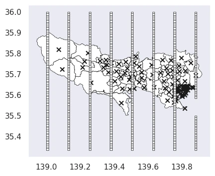
3次メッシュのポリゴンデータから一部のポリゴンを抽出する。
そして東京都の市町村区の代表点も抽出する。
可視化すると以下のような感じ。

# 一部のポリゴンを抽出
polyDf = dem4326[::10].reset_index(drop=True).copy()
fig = plt.figure(figsize=(6, 4))
ax = plt.subplot(1,1,1)
tokyo.plot(color='w', linewidth=0.5, edgecolor='k', ax=ax)
# 東京都の市町村区の代表点
tokyo.geometry.representative_point().plot(color='k', marker='x', ax=ax, markersize=6**2)
polyDf.plot(color='w', ax=ax, linewidth=0.5, edgecolor='k')
ax.grid(False)
plt.show()

ここから、東京都の各市町村区の代表点に最も近いポリゴンはどこかを計算する。sjoin_nearestを使えばOK。距離を正確に測るため、地域に合った投影座標系へ変換して実施する。

# インデックスをリセットし、新しいデータフレームとしてコピー
polyDf = dem4326[::10].reset_index(drop=True).copy()
# 結果を格納するための空のリストを初期化する。
tgtList=[]
# 市町村区の代表点（中心点）を一つずつループ処理
for target_point in tqdm(tokyo.geometry.representative_point()):
    # 現在の代表点（target_point）をGeoDataFrameに変換し、CRS情報を付与
    gdf_target = gpd.GeoDataFrame({'name': ['target']}, 
                               geometry=[target_point], 
                               crs=tokyo.crs)
    # 最近傍結合 (sjoin_nearest) を実行
    nearest = gpd.sjoin_nearest(
        # ターゲット点を、距離計算に適した投影座標系（EPSG:6677）に変換
        gdf_target.to_crs('EPSG:6677'),  # 投影座標系
        # 疎にしたデータ（polyDf）も同じ投影座標系に変換する。
        polyDf.to_crs('EPSG:6677'),  # 投影座標系
        # ターゲット点から最近傍の点までの距離を 'distance' 列に追加する。
        distance_col='distance'  # 距離列を追加
    # 結合後、結果を元の地理座標系（EPSG:4326）に戻す
    ).to_crs('EPSG:4326')

    # 'index_right'列には、polyDfにおける最近傍のレコードの元のインデックス番号が格納されている。
    # そのインデックス番号を使って、元のpolyDfから該当レコードを抽出する。
    tgt = polyDf.loc[nearest['index_right'].iloc[0]:nearest['index_right'].iloc[0]]
    # 抽出した結果をtgtListに追加する（インデックスは再度リセット）
    tgtList.append(tgt.reset_index(drop=True))
    
# ループで集めたすべての結果（tgtList）を結合し、一つのGeoDataFrameにする
tgt = pd.concat(tgtList).reset_index(drop=True)
display(tgt)

各市町村区の代表点に最も近いポリゴンを確認。

# 各市町村区の代表点に最も近いポリゴンを赤で表示
fig = plt.figure(figsize=(6, 4))
ax = plt.subplot(1,1,1)
tokyo.plot(color='w', linewidth=0.5, edgecolor='k', ax=ax)
# 各市町村区の代表点
tokyo.geometry.representative_point().plot(color='k', marker='x', ax=ax, markersize=6**2)
# ポリゴン
polyDf.plot(color='w', ax=ax, linewidth=0.5, edgecolor='k')
# 最も近いポリゴン
tgt.geometry.representative_point().plot(ax=ax, marker='.', markersize=6**2, color='r')
ax.grid(False)
plt.show()

円形に切り抜く

任意の位置の半径N km周辺を切り抜く。

データ読み込み。

# NDVI
rioNDVI = rio.open(os.path.join(dst_dir, 'NDVI_S2A_54SUE_20230107_0_L2A_B08_toCrsGdal.tif'))

# 標高3次メッシュ 
dem = gpd.read_file('../data/G04-a-11_5339-jgd_GML/G04-a-11_5339-jgd_ElevationAndSlopeAngleTertiaryMesh.shp')

# 行政区画 東京
# tokyo = gpd.read_file('../data/N03-20250101_13_GML/N03-20250101_13.shp')
# tokyo = tokyo[~tokyo['N03_004'].isin(['所属未定地', '大島町', '利島村', '新島村', '神津島村', '三宅村', '御蔵島村', '八丈町','青ヶ島村', '小笠原村'])]
# tokyo.to_crs('EPSG:4326').to_file('../data/N03-20250101_13_GML/N03-20250101_13_ep4326.geojson', driver='GeoJSON')
tokyo = gpd.read_file('../data/N03-20250101_13_GML/N03-20250101_13_ep4326.geojson')

# 土地利用細分メッシュ（ラスタ版）データ
landuse1 = rio.open('../data/L03-b-14_5339/L03-b-14_5339.tif')
landuse2 = rio.open('../data/L03-b-14_5340/L03-b-14_5340.tif')

# CRSのセット
# JGD2000: 日本測地系2000
dem4612 = dem.set_crs('EPSG:4612')
# CRSの変更
# WGS84
dem4326 = dem4612.to_crs('EPSG:4326')

任意の地点での、緯度経度1度あたりの距離を計算する。geopyのgeodesicを使用するとすぐに計算できる。
任意の地点をcoords_pointというPOINTオブジェクトとして定義しているとすると、以下のコードで計算できる。
東京だとおおよそ、1度あたり経度は90.5km、緯度は（どこでもほとんど同じだが）111.0kmとなる。

# 経度1度あたりの距離
dist1deg = geodesic((coords_point.y, coords_point.x), (coords_point.y, coords_point.x+1)).meters
# 緯度1度あたりの距離
dist1deg_lat = geodesic((coords_point.y, coords_point.x), (coords_point.y+1, coords_point.x)).meters

この計算をベースにコードを組む。sjoinとoverlayで切り抜き方が少し異なるのでどちらもできるようにしている。

def vector_crop_radius4326(gdf, coords_point, radius_km=10, method='sjoin'):
    # EPSG:4326での距離計算のため度をメートルに変換
    # 概算
    dist1deg = geodesic((coords_point.y, coords_point.x), (coords_point.y, coords_point.x+1)).meters
    dist1deg_lat = geodesic((coords_point.y, coords_point.x), (coords_point.y+1, coords_point.x)).meters
    print(f'経度1度あたりの距離概算{dist1deg} [m]')
    print(f'緯度1度あたりの距離概算{dist1deg_lat} [m]')
    radius_deg = (radius_km*1000)/dist1deg  # 概算での度単位変換
    radius_deg_lat = (radius_km*1000)/dist1deg_lat  # 概算での度単位変換
    print(f'距離{radius_km}kmに該当するdegree', '経度:', radius_deg, '緯度:', radius_deg_lat)

    # 緯度と経度で1度当たりの距離は異なるので処理をはさむ
    # affine変換でX方向とY方向に異なるスケールを適用して楕円に
    # x方向1として、y方向の縮尺
    xfact = 1
    yfact = radius_deg_lat/radius_deg

    # ポイント周辺円状のベクター
    buffered = gpd.GeoDataFrame(geometry=[coords_point], crs="EPSG:4326")
    buffered = buffered.buffer(radius_deg)
    # affine変換でX方向とY方向に異なるスケールを適用して楕円に
    buffered = buffered.geometry.map(lambda geom: shapely.affinity.scale(
        geom, 
        xfact=xfact,  # X方向のスケール
        yfact=yfact   # Y方向のスケール
    ))

    # 切り抜くベクター
    if method == 'sjoin':
        gdf_buffer = gdf.sjoin(gpd.GeoDataFrame(geometry=buffered, crs="EPSG:4326"), how='inner')
    elif method == 'overlay':
        gdf_buffer = gdf.overlay(gpd.GeoDataFrame(geometry=buffered, crs="EPSG:4326"), how='intersection')
    else:
        print('Crop method="sjoin"')
        gdf_buffer = gdf.sjoin(gpd.GeoDataFrame(geometry=buffered, crs="EPSG:4326"), how='inner')
    return gdf_buffer

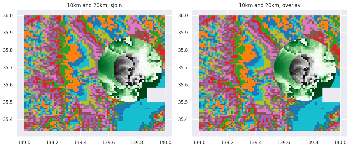
東京のとある市町村区の代表点の周囲10kmと20kmを切り抜く。
結果可視化。

# 周囲10kmで切り抜いたポリゴン
dem_buffer10 = vector_crop_radius4326(dem4326, coords_point, radius_km=10, method='sjoin')
# >> 経度1度あたりの距離概算90517.95070298456 [m]
# >> 緯度1度あたりの距離概算110962.48443561903 [m]
# >> 距離10kmに該当するdegree 経度: 0.11047532475423441 緯度: 0.09012054885813275
# 周囲20kmで切り抜いたポリゴン
dem_buffer20 = vector_crop_radius4326(dem4326, coords_point, radius_km=20, method='sjoin')
# >> 経度1度あたりの距離概算90517.95070298456 [m]
# >> 緯度1度あたりの距離概算110962.48443561903 [m]
# >> 距離20kmに該当するdegree 経度: 0.22095064950846882 緯度: 0.1802410977162655

fig = plt.figure(figsize=(12, 6))
ax = plt.subplot(1,2,1)
# 元のベクター
dem4326.plot(column='G04a_002', linewidth=0, ax=ax, zorder=1)
# 20kmで切り抜いたベクター
dem_buffer20.plot(column='G04a_002', linewidth=0, ax=ax, zorder=2, cmap='Greens')
# 10kmで切り抜いたベクター
dem_buffer10.plot(column='G04a_002', linewidth=0, ax=ax, zorder=3, cmap='binary')
# とある市町村区の代表点 
gpd.GeoDataFrame(geometry=[coords_point], crs="EPSG:4326").plot(ax=ax, color='k', edgecolor='w', markersize=10**2, zorder=4)
ax.set_title('10km and 20km, sjoin')

dem_buffer10 = vector_crop_radius4326(dem4326, coords_point, radius_km=10, method='overlay')
# >> 経度1度あたりの距離概算90517.95070298456 [m]
# >> 緯度1度あたりの距離概算110962.48443561903 [m]
# >> 距離10kmに該当するdegree 経度: 0.11047532475423441 緯度: 0.09012054885813275
dem_buffer20 = vector_crop_radius4326(dem4326, coords_point, radius_km=20, method='overlay')
# >> 経度1度あたりの距離概算90517.95070298456 [m]
# >> 緯度1度あたりの距離概算110962.48443561903 [m]
# >> 距離20kmに該当するdegree 経度: 0.22095064950846882 緯度: 0.1802410977162655

ax = plt.subplot(1,2,2)
# 元のベクター
dem4326.plot(column='G04a_002', linewidth=0, ax=ax, zorder=1)
# 20kmで切り抜いたベクター
dem_buffer20.plot(column='G04a_002', linewidth=0, ax=ax, zorder=2, cmap='Greens')
# 10kmで切り抜いたベクター
dem_buffer10.plot(column='G04a_002', linewidth=0, ax=ax, zorder=3, cmap='binary')
# とある市町村区の代表点 
gpd.GeoDataFrame(geometry=[coords_point], crs="EPSG:4326").plot(ax=ax, color='k', edgecolor='w', markersize=10**2, zorder=4)
ax.set_title('10km and 20km, overlay')
plt.tight_layout()
plt.show()

空間可視化のコード

データ読み込み。

# NDVI
rioNDVI = rio.open(os.path.join(dst_dir, 'NDVI_S2A_54SUE_20230107_0_L2A_B08_toCrsGdal.tif'))

# 標高3次メッシュ 
dem = gpd.read_file('../data/G04-a-11_5339-jgd_GML/G04-a-11_5339-jgd_ElevationAndSlopeAngleTertiaryMesh.shp')

# 行政区画 東京
# tokyo = gpd.read_file('../data/N03-20250101_13_GML/N03-20250101_13.shp')
# tokyo = tokyo[~tokyo['N03_004'].isin(['所属未定地', '大島町', '利島村', '新島村', '神津島村', '三宅村', '御蔵島村', '八丈町','青ヶ島村', '小笠原村'])]
# tokyo.to_crs('EPSG:4326').to_file('../data/N03-20250101_13_GML/N03-20250101_13_ep4326.geojson', driver='GeoJSON')
tokyo = gpd.read_file('../data/N03-20250101_13_GML/N03-20250101_13_ep4326.geojson')

# 土地利用細分メッシュ（ラスタ版）データ
landuse1 = rio.open('../data/L03-b-14_5339/L03-b-14_5339.tif')
landuse2 = rio.open('../data/L03-b-14_5340/L03-b-14_5340.tif')

# CRSのセット
# JGD2000: 日本測地系2000
dem4612 = dem.set_crs('EPSG:4612')
# CRSの変更
# WGS84
dem4326 = dem4612.to_crs('EPSG:4326')
dem4326['G04a_002'] = pd.to_numeric(dem4326['G04a_002'], errors='coerce')

地図としてベクターやラスターを可視化するときのベース関数。フォントサイズの設定やカラーバーの設定などを行う。

# plotの設定関数
def plot_config(ax, legend=True, style='plain', fontsize=10, rotation=None, grid=False, leg_fontsize='8', bbox_to_anchor=None, loc=None, borderaxespad=None, facecolor=None, edgecolor=None):
    plt.rcParams['font.family'] = prop.get_name() #全体のフォントを設定
    plt.setp(ax.get_xticklabels(), fontsize=fontsize, rotation=rotation)
    plt.setp(ax.get_yticklabels(), fontsize=fontsize)
    ax.yaxis.offsetText.set_fontsize(fontsize)
    ax.yaxis.set_major_formatter(ptick.ScalarFormatter(useMathText=True))
    ax.ticklabel_format(style=style, axis='y', scilimits=(0,0))
    ax.grid(grid)
    if legend:
        ax.legend(bbox_to_anchor=bbox_to_anchor, loc=loc, borderaxespad=borderaxespad, facecolor=facecolor, edgecolor=edgecolor)
        plt.setp(ax.get_legend().get_texts(), fontsize=leg_fontsize)

# ラスター用カラーバー関数
def raster_cbar(img, labelsize=10):
    divider = mpl_toolkits.axes_grid1.make_axes_locatable(ax)
    cax = divider.append_axes('right', '5%', pad=0.)
    cbar = plt.colorbar(img, cax=cax)
    cbar.ax.tick_params(labelsize=labelsize)
    return cax, cbar

def raster_cbar_ax(ax, img, labelsize=10):
    divider = mpl_toolkits.axes_grid1.make_axes_locatable(ax)
    cax = divider.append_axes('right', '5%', pad=0.)
    cbar = plt.colorbar(img, cax=cax)
    cbar.ax.tick_params(labelsize=labelsize)
    return cax, cbar
    
# ベクターデータ用カラーバー関数
def vec_cbar():
    divider = mpl_toolkits.axes_grid1.make_axes_locatable(ax)
    cax = divider.append_axes('right', '4%', pad=0.)
    return cax

def combine_colormaps(*cmaps, samples=128, ranges=None):
    """
    任意の数のカラーマップを組み合わせる関数

    Parameters:
    *cmaps : matplotlib.colors.Colormap
        組み合わせるカラーマップ
    samples : int, optional
        各カラーマップから抽出するサンプル数 (デフォルト: 128)
    ranges : list of tuple, optional
        各カラーマップの範囲 [(start1, end1), (start2, end2), ...] (デフォルト: None)

    Returns:
    matplotlib.colors.ListedColormap
        組み合わされた新しいカラーマップ

    example:
    # 使用例
    cmap1 = plt.cm.autumn
    cmap2 = plt.cm.winter
    cmap3 = plt.cm.binary
    # カスタム範囲で組み合わせる
    custom_combined_cmap = combine_colormaps(cmap1, cmap2, cmap3, 
                                             ranges=[(0.5, 1), (0.5, 1), (0.05, 0.2)])
    """
    if ranges is None:
        ranges = [(0, 1)] * len(cmaps)
    
    if len(ranges) != len(cmaps):
        raise ValueError("ranges の数は cmaps の数と一致する必要があります")

    newcolors = []
    for cmap, (start, end) in zip(cmaps, ranges):
        newcolors.append(cmap(np.linspace(start, end, samples)))

    combined_colors = np.vstack(newcolors)
    return matplotlib.colors.ListedColormap(combined_colors, name='combined_cmap')

ラスター可視化

数値のカラーバー付き　ラスター

tif_f = os.path.join(dst_dir, 'NDVI_S2A_54SUE_20230107_0_L2A_B08_toCrsGdal.tif')

fig = plt.figure(figsize=(12, 6))
ax = fig.add_subplot(1,1,1)
retted = show(rio.open(tif_f), cmap='Spectral_r', ax=ax, vmin=-1, vmax=1, zorder=1)
# imageオブジェクト
img = retted.get_images()[0]
# imageオブジェクトにカラーバー追加
cax, cbar = raster_cbar(img, labelsize=10)
# 東京都区画
tokyo.plot(facecolor='None', linewidth=3, edgecolor='w', ax=ax, zorder=2)
tokyo.plot(facecolor='None', linewidth=1, edgecolor='k', ax=ax, zorder=2)
ax.set_xlim(tokyo.total_bounds[0], tokyo.total_bounds[2])
ax.set_ylim(tokyo.total_bounds[1], tokyo.total_bounds[3])
plot_config(ax, legend=False
            , style='plain', fontsize=10, rotation=None
            , grid=False
            , leg_fontsize='8', bbox_to_anchor=None, loc=None, borderaxespad=None
            , facecolor=None, edgecolor=None)
plt.show()

カテゴリーのカラーバー付き　ラスター

NDVIが低、中、高の3段階で示されたラスターデータを可視化する。（値としては0,1,2で表現されている。）

leg_dic = {0:'低',1:'中',2:'高'}  # 3段階の凡例
tif_f = temp_dir+'/Category_NDVI_S2A_54SUE_20230107_0_L2A_B08_toCrsGdal.tif'

fig = plt.figure(figsize=(12, 6))
ax = fig.add_subplot(1,1,1)
retted = show(rio.open(tif_f), cmap='Spectral_r', ax=ax, zorder=1)
# imageオブジェクト
img = retted.get_images()[0]
# imageオブジェクトにカラーバー追加
cax, cbar = raster_cbar(img, labelsize=10)
cax.set_yticks([c for c in leg_dic.keys()])
cax.set_yticklabels([c for c in leg_dic.values()])
# 東京都区画
tokyo.plot(facecolor='None', linewidth=3, edgecolor='w', ax=ax, zorder=2)
tokyo.plot(facecolor='None', linewidth=1, edgecolor='k', ax=ax, zorder=2)
ax.set_xlim(tokyo.total_bounds[0], tokyo.total_bounds[2])
ax.set_ylim(tokyo.total_bounds[1], tokyo.total_bounds[3])
plot_config(ax, legend=False
            , style='plain', fontsize=10, rotation=None
            , grid=False
            , leg_fontsize='8', bbox_to_anchor=None, loc=None, borderaxespad=None
            , facecolor=None, edgecolor=None)
plt.show()

rasterioのshowを使わない方法

ax.imshow()でも描画可能。

leg_dic = {0:'低',1:'中',2:'高'}  # 3段階の凡例
tif_f = temp_dir+'/Category_NDVI_S2A_54SUE_20230107_0_L2A_B08_toCrsGdal.tif'
# TIFの情報取得
with rio.open(tif_f) as src:
    data = src.read(1)
    bounds = src.bounds
    
fig = plt.figure(figsize=(12, 6))
ax = fig.add_subplot(1,1,1)
# imageオブジェクト
img = ax.imshow(data, cmap='Spectral_r', extent=[bounds.left, bounds.right, bounds.bottom, bounds.top], zorder=1)
# imageオブジェクトにカラーバー追加
cax, cbar = raster_cbar(img, labelsize=10)
cax.set_yticks([c for c in leg_dic.keys()])
cax.set_yticklabels([c for c in leg_dic.values()])
# 東京都区画
tokyo.plot(facecolor='None', linewidth=3, edgecolor='w', ax=ax, zorder=2)
tokyo.plot(facecolor='None', linewidth=1, edgecolor='k', ax=ax, zorder=2)
ax.set_xlim(tokyo.total_bounds[0], tokyo.total_bounds[2])
ax.set_ylim(tokyo.total_bounds[1], tokyo.total_bounds[3])
plot_config(ax, legend=False
            , style='plain', fontsize=10, rotation=None
            , grid=False
            , leg_fontsize='8', bbox_to_anchor=None, loc=None, borderaxespad=None
            , facecolor=None, edgecolor=None)
plt.show()

ベクター可視化

数値のカラーバー付き　ベクター

fig = plt.figure(figsize=(12, 6))
ax = fig.add_subplot(1,2,1)
cax = vec_cbar()
# 標高3次メッシュ
dem4326.plot(linewidth=0.5, edgecolor='k', column='G04a_002', ax=ax, cax=cax, legend=True, cmap='nipy_spectral')
# 東京都区画
tokyo.plot(facecolor='None', linewidth=3, edgecolor='w', ax=ax, zorder=2)
tokyo.plot(facecolor='None', linewidth=1, edgecolor='k', ax=ax, zorder=2)
plot_config(ax, legend=False
            , style='plain', fontsize=10, rotation=None
            , grid=False
            , leg_fontsize='8', bbox_to_anchor=None, loc=None, borderaxespad=None
            , facecolor=None, edgecolor=None)

ax = fig.add_subplot(1,2,2)
cax = vec_cbar()
# 標高3次メッシュ
# linewidth=0
dem4326.plot(linewidth=0., edgecolor='k', column='G04a_002', ax=ax, cax=cax, legend=True, cmap='nipy_spectral')
# 東京都区画
tokyo.plot(facecolor='None', linewidth=3, edgecolor='w', ax=ax, zorder=2)
tokyo.plot(facecolor='None', linewidth=1, edgecolor='k', ax=ax, zorder=2)
plot_config(ax, legend=False
            , style='plain', fontsize=10, rotation=None
            , grid=False
            , leg_fontsize='8', bbox_to_anchor=None, loc=None, borderaxespad=None
            , facecolor=None, edgecolor=None)
plt.show()

右は標高のlinewidth=0にしているだけ。

カテゴリーの凡例付き　ベクター

標高を4段階で表した列を作成して可視化。

s_cut, bins = pd.cut(dem4326['G04a_002'], bins=5, retbins=True, labels=False)
dem4326['DEM_category'] = s_cut
categories = {0.0:'超低', 1.0:'低', 2.0:'普通', 3.0:'高', 4.0:'超高'}
dem4326['DEM_category_str'] = dem4326['DEM_category'].replace(categories)

fig = plt.figure(figsize=(12, 6))
ax = fig.add_subplot(1,2,1)
# 標高3次メッシュ
dem4326.plot(linewidth=0.5, edgecolor='k', column='DEM_category_str'
             , ax=ax, legend=True, cmap='nipy_spectral'
             , categorical=True, categories=['超低', '低', '普通', '高', '超高'])
# 東京都区画
tokyo.plot(facecolor='None', linewidth=3, edgecolor='w', ax=ax, zorder=2)
tokyo.plot(facecolor='None', linewidth=1, edgecolor='k', ax=ax, zorder=2)
plot_config(ax, legend=False
            , style='plain', fontsize=10, rotation=None
            , grid=False
            , leg_fontsize='8', bbox_to_anchor=None, loc=None, borderaxespad=None
            , facecolor=None, edgecolor=None)

ax = fig.add_subplot(1,2,2)
# 標高3次メッシュ
# linewidth=0
dem4326.plot(linewidth=0., edgecolor='k', column='DEM_category_str'
             , ax=ax, legend=True, cmap='nipy_spectral'
             , categorical=True, categories=['超低', '低', '普通', '高', '超高'])
# 東京都区画
tokyo.plot(facecolor='None', linewidth=3, edgecolor='w', ax=ax, zorder=2)
tokyo.plot(facecolor='None', linewidth=1, edgecolor='k', ax=ax, zorder=2)
plot_config(ax, legend=False
            , style='plain', fontsize=10, rotation=None
            , grid=False
            , leg_fontsize='8', bbox_to_anchor=None, loc=None, borderaxespad=None
            , facecolor=None, edgecolor=None)
plt.show()

右は標高のlinewidth=0にしているだけ。

カテゴリーのカラーバー付き　ベクター

凡例ではなくカラーバーで表現。

s_cut, bins = pd.cut(dem4326['G04a_002'], bins=5, retbins=True, labels=False)
dem4326['DEM_category'] = s_cut
categories = {0.0:'超低', 1.0:'低', 2.0:'普通', 3.0:'高', 4.0:'超高'}
dem4326['DEM_category_str'] = dem4326['DEM_category'].replace(categories)

fig = plt.figure(figsize=(12, 6))
ax = fig.add_subplot(1,2,1)
# 標高3次メッシュ
cax = vec_cbar()
dem4326.plot(linewidth=0.5, edgecolor='k', column='DEM_category'
             , ax=ax, cax=cax, legend=True, cmap='nipy_spectral')
cax.set_yticks([c for c in categories.keys()])
cax.set_yticklabels([c for c in categories.values()])
# 東京都区画
tokyo.plot(facecolor='None', linewidth=3, edgecolor='w', ax=ax, zorder=2)
tokyo.plot(facecolor='None', linewidth=1, edgecolor='k', ax=ax, zorder=2)
plot_config(ax, legend=False
            , style='plain', fontsize=10, rotation=None
            , grid=False
            , leg_fontsize='8', bbox_to_anchor=None, loc=None, borderaxespad=None
            , facecolor=None, edgecolor=None)

ax = fig.add_subplot(1,2,2)
# 標高3次メッシュ
# linewidth=0
cax = vec_cbar()
dem4326.plot(linewidth=0., edgecolor='k', column='DEM_category'
             , ax=ax, cax=cax, legend=True, cmap='nipy_spectral')
cax.set_yticks([c for c in categories.keys()])
cax.set_yticklabels([c for c in categories.values()])
# 東京都区画
tokyo.plot(facecolor='None', linewidth=3, edgecolor='w', ax=ax, zorder=2)
tokyo.plot(facecolor='None', linewidth=1, edgecolor='k', ax=ax, zorder=2)
plot_config(ax, legend=False
            , style='plain', fontsize=10, rotation=None
            , grid=False
            , leg_fontsize='8', bbox_to_anchor=None, loc=None, borderaxespad=None
            , facecolor=None, edgecolor=None)
plt.show()

右は標高のlinewidth=0にしているだけ。

おわりに

他に書くべき処理が出てきたら追加していくことにする。

以上！

You get articles that match your needs
You can efficiently read back useful information
You can use dark theme

What you can do with signing up

Pythonによる地理空間データのハンドリングまとめ

はじめに

参考

import

使用データ

ラスターの取り扱い

CRSの変更

rasterio

gdal コマンド

結果可視化

リサンプリング

rasterio (resampling & crop)

rasterio (resampling)

gdal コマンド (resampling)

結果可視化

クロップ

rasterio：ポリゴンの範囲に切り取る

rasterio：bboxの範囲に切り取る

gdalコマンド：ポリゴンの範囲に切り取る

gdalコマンド：bboxの範囲に切り取る

結果可視化

マージ

rasterio

gdalコマンド

結果可視化

Nodata値変更

指数計算

ラスターからベクターに変換

rasterio：rio.features.shapesを使用

rasterio：全ピクセルをポリゴン化

結果可視化

円形に切り抜く

ベクターの取り扱い

CRSの変更

クロップ

ベクターからラスターに変換

ポリゴン内のラスター値の統計量（ゾーン統計）

rasterstats.zonal_statsを使用

exactextract.exact_extractを使用

2つのアプローチの比較

結果可視化

ポイントデータの位置に対応するラスター値を取得

メッシュコード取得

任意のPOINTに最も近いgeometryを取得する

円形に切り抜く

空間可視化のコード

ラスター可視化

数値のカラーバー付き ラスター

カテゴリーのカラーバー付き ラスター

rasterioのshowを使わない方法

ベクター可視化

数値のカラーバー付き ベクター

カテゴリーの凡例付き ベクター

カテゴリーのカラーバー付き ベクター

おわりに

数値のカラーバー付き　ラスター

カテゴリーのカラーバー付き　ラスター

数値のカラーバー付き　ベクター

カテゴリーの凡例付き　ベクター

カテゴリーのカラーバー付き　ベクター