優勝コードから学ぶ―メルカリコンペ編①―

はじめに

Kaggleの勉強をするにあたり、過去のコンペで１位をとった人のコードから勉強しようということで、今回はメルカリコンペの1位の方のコードを題材に勉強しました。

学んだこと

・コンテキストマネージャを使った時間計測
・Pipeline化とFunctionTransformer
・TF-IDF, itemgetter, TfidfVectorizer
・4層MLP(Multilayer perceptron)でも精度がでる
・partialを使用してy_trainは固定してx_trainだけ変える

メルカリコンペ概要

内容

出品時の妥当な値段を予測するモデルの作成

意義

出品時に商品情報から適切な値段を自動的に提示することで出品時の手間を削減する。出品が簡単になる。

背景

メルカリの相場から外れて、高い値段で出品した場合売れない
逆にメルカリの相場より低い値段で出品してしまった場合、お客さまが損をする

コンペの制約

カーネルコンペ：ソースコード自体をKaggleに提出。提出するとKaggle上で実行されてスコアが算出される。
計算機資源と計算時間の制約がある

CPU: 4 cores
Memory: 16GB
Disk: 1GB
制限時間: １時間
GPU: なし

評価

RMLSE：Root Mean Squared Logarithmic Error
スコアが低ければ低いほど、小さい誤差で値段を推定できたことになる

一位の方のモデルはRMLSE: 0.3875

使用データ

列名	説明
name	商品名
item_condition_id	中古、新品など、商品の状態。(1~5)、大きい方が状態が良い。
category_name	大まかなカテゴリ/詳細なカテゴリ/より詳細なカテゴリ
brand_name	ブランド名。例: Nike, Apple
price	過去の販売価格(USD)
shipping	送料を出品者か購入者のどちらが支払うか。1 -> 出品者が払う, 0 -> 購入者が払う。
item_description	商品の詳細

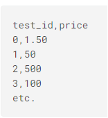
出力形式

Test_idとprice

１位のコードの要点

・100行という短さ。シンプル。
・4層MLP。精度でている。この時代はまだニューラルネットワークは使用されていなかった？
・TF-IDF。 df['name'].fillna('') + ' ' + df['brand_name'].fillna('')で文字列を結合したことで精度UP?
・y_trainの標準化
・4コアで4モデルを学習->アンサンブル

教師データの準備

各処理にかかる時間の計測

1時間との制約があるため、どこの処理でどれだけの時間を使っているか計測する工夫が入れられている。
各処理の箇所にwith timerが入れられている。with timerの説明。

教師データの作成

qiita.rb

 with timer('process train'):
# ロード
        train = pd.read_table('../input/train.tsv')
# 0ドルのpriceが存在しているためはじいている
        train = train[train['price'] > 0].reset_index(drop=True)
# データを学習用と検証用で分割するための準備
        cv = KFold(n_splits=20, shuffle=True, random_state=42)
# データを学習用と検証用で分割
# .split()でイテラブルなオブジェクトが帰ってくる。学習用の「インデックスと検証用のインデックスが取り出せる。
# next()でイテレータ内から要素を取得
        train_ids, valid_ids = next(cv.split(train))
# 取得したインデックスで学習と検証用に分割
        train, valid = train.iloc[train_ids], train.iloc[valid_ids]
# 価格は1行n列をn行1列に変換。log(a+1)で変換。正規化
        y_train = y_scaler.fit_transform(np.log1p(train['price'].values.reshape(-1, 1)))
# パイプラインで処理
        X_train = vectorizer.fit_transform(preprocess(train)).astype(np.float32)
        print(f'X_train: {X_train.shape} of {X_train.dtype}')
        del train
# 検証用データも同様に前処理
  with timer('process valid'):
        X_valid = vectorizer.transform(preprocess(valid)).astype(np.float32)

前処理

ブランド名には欠損値があるため、空白に置き換えている。そのうえで、商品名とブランド名を結合している。あとでTF-IDFしやすいようにする為。新しくtextという要素を作っている。'name', 'text', 'shipping', 'item_condition_id'はこの後のPipelineの処理で使用する。

qiita.rb

def preprocess(df: pd.DataFrame) -> pd.DataFrame:
    df['name'] = df['name'].fillna('') + ' ' + df['brand_name'].fillna('')
    df['text'] = (df['item_description'].fillna('') + ' ' + df['name'] + ' ' + df['category_name'].fillna(''))
    return df[['name', 'text', 'shipping', 'item_condition_id']]

文字の抽出とTF-IDFの算出を一連の流れで行えるようにPipeline化している。

PipeLineの説明。

qiita.rb

def on_field(f: str, *vec) -> Pipeline:
    return make_pipeline(FunctionTransformer(itemgetter(f), validate=False), *vec)

def to_records(df: pd.DataFrame) -> List[Dict]:
    return df.to_dict(orient='records')

 vectorizer = make_union(
        on_field('name', Tfidf(max_features=100000, token_pattern='\w+')),
        on_field('text', Tfidf(max_features=100000, token_pattern='\w+', ngram_range=(1, 2))),
        on_field(['shipping', 'item_condition_id'],
                 FunctionTransformer(to_records, validate=False), DictVectorizer()),
        n_jobs=4)
    y_scaler = StandardScaler()

 X_train = vectorizer.fit_transform(preprocess(train)).astype(np.float32)

文字種類分(200000)のスコア（Bag of Words）と'shipping', 'item_condition_id'のスコア合計200002が出力となる。

学習

4コア4スレッドで学習し、その後平均をとってアンサンブルを行っている。
学習の際はy_trainはpartialで固定してxsだけを変えている。

qiita.rb

def fit_predict(xs, y_train) -> np.ndarray:
    X_train, X_test = xs
    config = tf.ConfigProto(
        intra_op_parallelism_threads=1, use_per_session_threads=1, inter_op_parallelism_threads=1)
    with tf.Session(graph=tf.Graph(), config=config) as sess, timer('fit_predict'):
        ks.backend.set_session(sess)
        model_in = ks.Input(shape=(X_train.shape[1],), dtype='float32', sparse=True)#MLPの設計
        out = ks.layers.Dense(192, activation='relu')(model_in)
        out = ks.layers.Dense(64, activation='relu')(out)
        out = ks.layers.Dense(64, activation='relu')(out)
        out = ks.layers.Dense(1)(out)
        model = ks.Model(model_in, out)
        model.compile(loss='mean_squared_error', optimizer=ks.optimizers.Adam(lr=3e-3))
        for i in range(3):#3エポック
            with timer(f'epoch {i + 1}'):
                model.fit(x=X_train, y=y_train, batch_size=2**(11 + i), epochs=1, verbose=0)#バッチサイズは指数関数的に増加させる
        return model.predict(X_test)[:, 0]#予想を返す


 with ThreadPool(processes=4) as pool: #4つのスレッドにする
        Xb_train, Xb_valid = [x.astype(np.bool).astype(np.float32) for x in [X_train, X_valid]]
        xs = [[Xb_train, Xb_valid], [X_train, X_valid]] * 2
        y_pred = np.mean(pool.map(partial(fit_predict, y_train=y_train), xs), axis=0)#4コアで学習したものの平均をとっている
    y_pred = np.expm1(y_scaler.inverse_transform(y_pred.reshape(-1, 1))[:, 0])#logで変換していたものを価格に戻す
    print('Valid RMSLE: {:.4f}'.format(np.sqrt(mean_squared_log_error(valid['price'], y_pred))))

参考

参考①
参考②
参考③
参考④
BRONZE取得者の手法
メルカリHP