
はじめに
以前の記事[1]では、電源・線路・リアクトル負荷・電力用コンデンサからなる簡単な回路を用い、コンデンサが受電端電圧と無効電力のやり取りに与える影響を確認した。今回は同じく一機無限大母線に接続された受電端を対象に、受電端の有効電力 $P$ を増加させたときに電圧 $V$ がどこで限界を迎えるかを、いわゆるノーズカーブ(P-V曲線)[2, 3]として調べる。
具体的には、次の三つを変数とした P-V 曲線の族を描く。
- 送電線のインダクタンス $L$(リアクタンス $X=\omega L$)
- 負荷の力率 $\cos\theta$
- 調相用コンデンサの静電容量 $C$
ノーズの先端(鼻先)は、その条件下で定常的に送れる有効電力の上限に相当する。先端より低電圧側にも数学的な解(低電圧枝)は存在するが、実運用としては不安定になりやすい領域である。本記事は実系統の設計値を決めるものではなく、電圧安定性の基本的な振る舞いを学ぶための簡略化モデルによる数値実験である。
なお本記事の受電端方程式は、後述するように $V^2$ についての2次方程式に帰着する。これにより、反復法(潮流計算のニュートン法など)を使わずに、両方の電圧枝(高電圧枝・低電圧枝)を一度に閉形式で求めることができる。
この記事で扱うモデル
電源電圧を基準位相の複素数 $\dot E=E\angle0$(一定)とし、送電線インピーダンスを
$$
\dot Z=R+jX,\qquad X=\omega L
$$
とする。受電端には、指定した有効電力 $P$ と遅れ力率角 $\theta$ の負荷、および並列の調相用コンデンサ $C$ を接続する。回路構成は文献[1]の無効電力供給・消費モデルと同等である。
無限大母線                         受電端
E∠0 ───── R + jωL ─────●── PQ負荷(P, cosθ)
                            └── 調相用コンデンサ C
前回の記事[1]では負荷を固定インピーダンスとして扱ったが、今回は $P$ と力率を指定する PQ 負荷を用いる。固定インピーダンスのままでは受電端電圧の変化に伴って消費電力自体も変わってしまうため、「$P$ を増やしていったときに $V$ がどう追従するか」というノーズカーブの問いには使えない。
定式化
受電端電圧を $\dot V=V\angle0$(基準位相)とすると、送電端は $\dot E=E\angle\delta$ と表せる($\delta$ は送受電端間の位相差、未知数)。線路インピーダンスを極形式で
$$
\dot Z=|Z|\angle\varphi,\qquad |Z|=\sqrt{R^2+X^2},\quad \varphi=\tan^{-1}\frac{X}{R}
$$
と書くと、受電端に流れ込む電流 $\dot I=(\dot E-\dot V)/\dot Z$ から、受電端の複素電力 $S=\dot V\dot I^{*}=P+jQ$ は次のように展開できる。
$$
P=\frac{VE}{|Z|}\cos(\varphi-\delta)-\frac{V^2}{|Z|}\cos\varphi \tag{1}
$$
$$
Q=\frac{VE}{|Z|}\sin(\varphi-\delta)-\frac{V^2}{|Z|}\sin\varphi \tag{2}
$$
($R=0$ とすれば $\varphi=90^\circ$ となり、教科書でよく見る $P=\dfrac{EV}{X}\sin\delta$、$Q=\dfrac{EV\cos\delta-V^2}{X}$ に一致する。)
負荷の無効電力は、遅れを正として $Q_{\mathrm{load}}=P\tan\theta$ である。理想コンデンサが受電端電圧に対して供給する無効電力は $Q_C=\omega C,V^2$(進み)であるため、線路側から見た受電端の正味無効電力は
$$
Q=P\tan\theta-\omega C V^2 \tag{3}
$$
となる。式(1)(2)(3)には未知数が $V,\delta$ の二つしかないので、$\delta$ を消去すれば $V$ だけの方程式が得られる。式(1)より
$$
\frac{VE}{|Z|}\cos(\varphi-\delta)=P+\frac{V^2}{|Z|}\cos\varphi \tag{1'}
$$
式(2)(3)より
$$
\frac{VE}{|Z|}\sin(\varphi-\delta)=P\tan\theta-\omega C V^2+\frac{V^2}{|Z|}\sin\varphi \tag{2'}
$$
(1')と(2')をそれぞれ2乗して足し合わせると、$\cos^2+\sin^2=1$ により左辺は $\left(\dfrac{VE}{|Z|}\right)^2$ にまとまり、$\delta$ が消去される。整理すると、$w\equiv V^2$ についての2次方程式
$$
A,w^2+B(P),w+C_{!*}(P)=0 \tag{4}
$$
$$
A=c_1^2+(s_1-\omega C)^2,\qquad
c_1=\frac{\cos\varphi}{|Z|},\ \ s_1=\frac{\sin\varphi}{|Z|}
$$
$$
B(P)=2P\bigl[c_1+\tan\theta,(s_1-\omega C)\bigr]-\frac{E^2}{|Z|^2}
$$
$$
C_{!*}(P)=P^2\sec^2\theta
$$
を得る。$A$ は $P$ に依存しない定数、$B$ は $P$ の1次式、$C_{!*}$ は $P$ の2次式である。したがって、与えた $P,,X(=\omega L),,\theta,,C$ に対して、解の公式
$$
V^2=\frac{-B\pm\sqrt{B^2-4AC_{!*}}}{2A}
$$
から直接 $V$ の二つの枝($+$: 高電圧枝、$-$: 低電圧枝)が求まる。判別式 $B^2-4AC_{!}$ が負になる $P$ では実数解が存在せず、それが定常的に送電できる有効電力の上限(ノーズの先端)である。$A,B,C_{!}$ が $P$ の高々2次式であることから、判別式もまた $P$ についての2次式であり、ノーズ先端の $P$ は原理的には解析的に求められる(本記事では実装を単純にするため $P$ を細かく走査して判別式の符号が変わる点を探す)。
計算の進め方
- $E,R,f$ を固定し、$L,\theta,C$ のうち掃引したい一つ以外を固定する。
- $P$ の配列に対して式(4)を評価し、判別式が非負の区間で高電圧枝・低電圧枝の $V$ を同時に求める。
- 判別式が負に転じる直前の $P$ をノーズ先端の近似値として記録する。
- 上記を $L,\theta,C$ それぞれについて複数値で繰り返し、色分けした P-V 曲線群として重ね描きする。
反復法による潮流計算(ニュートン法や scipy.optimize.root など)とは異なり、初期値の選び方や収束判定に悩む必要がなく、低電圧枝も高電圧枝と同じ手間で得られる点が本モデルの利点である。
Python実装
必要なライブラリは NumPy と Matplotlib のみである。
import numpy as np

def branch_voltages(P, E, R, L, f, theta, C):
    """式(4)を解いて高電圧枝・低電圧枝の V を返す。"""
    omega = 2.0 * np.pi * f
    X = omega * L
    absZ = np.hypot(R, X)
    phi = np.arctan2(X, R)
    c1 = np.cos(phi) / absZ
    s1 = np.sin(phi) / absZ
    tan_th = np.tan(theta)
    k = omega * C

    A = c1**2 + (s1 - k)**2
    B = 2.0 * P * (c1 + tan_th * (s1 - k)) - E**2 / absZ**2
    Cc = (P**2) * (1.0 + tan_th**2)

    disc = B**2 - 4.0 * A * Cc
    sqrt_disc = np.sqrt(np.where(disc >= 0.0, disc, np.nan))
    w_high = (-B + sqrt_disc) / (2.0 * A)
    w_low = (-B - sqrt_disc) / (2.0 * A)
    V_high = np.sqrt(np.where(w_high >= 0.0, w_high, np.nan))
    V_low = np.sqrt(np.where(w_low >= 0.0, w_low, np.nan))
    return V_high, V_low
$P$ を配列で与えれば、NumPy のブロードキャストにより高電圧枝・低電圧枝が一度に求まる。反復も継続法も不要である。
P_values = np.linspace(1.0, 30_000.0, 4000)
V_high, V_low = branch_voltages(
    P_values, E=100.0, R=0.10, L=1.0e-3,
    f=50.0, theta=np.deg2rad(30.0), C=100e-6)
描画する三つのP-V曲線群
$E,R,f$ を固定し、$L,\theta,C$ のうち一つを掃引したときの P-V 曲線群を示す。各図で実線が高電圧枝、破線が低電圧枝、丸印が判別式の符号が変わる直前の点(ノーズ先端の近似位置)である。
1. P-V-L(P-V-X)
$L$ を 0.4〜1.6 mH の範囲で掃引した(他は基準値: $\theta=30^\circ$, $C=100,\mu\mathrm F$)。
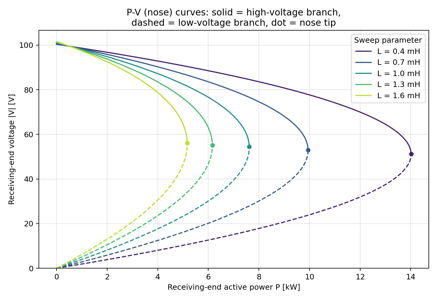
線路リアクタンス $X=\omega L$ が大きいほど電圧降下が大きくなり、ノーズの先端は小さい $P$ 側・低い $V$ 側へ移動する。これは、同じ有効・無効電力を送るために必要な位相差 $\delta$ と電圧降下が、$X$ に比例して増えるためである。
2. P-V-θ(力率)
力率角 $\theta$ を $10^\circ$〜$50^\circ$($\cos\theta\simeq0.98$〜$0.64$)の範囲で掃引した(他は基準値: $L=1.0,\mathrm{mH}$, $C=100,\mu\mathrm F$)。
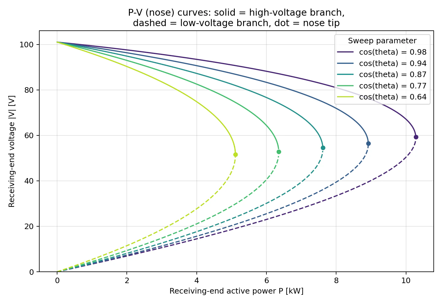
遅れ力率角が大きいほど、負荷が要求する無効電力 $P\tan\theta$ が増える。線路はその無効電力も一緒に運ばなければならないため、電圧維持が難しくなり、ノーズ先端は小さい $P$ 側へ移動する。力率改善が電圧安定性にも寄与することが、この図から視覚的に確認できる。
3. P-V-C(調相用コンデンサ)
調相用コンデンサの容量 $C$ を 0〜200 $\mu\mathrm F$ の範囲で掃引した(他は基準値: $L=1.0,\mathrm{mH}$, $\theta=30^\circ$)。
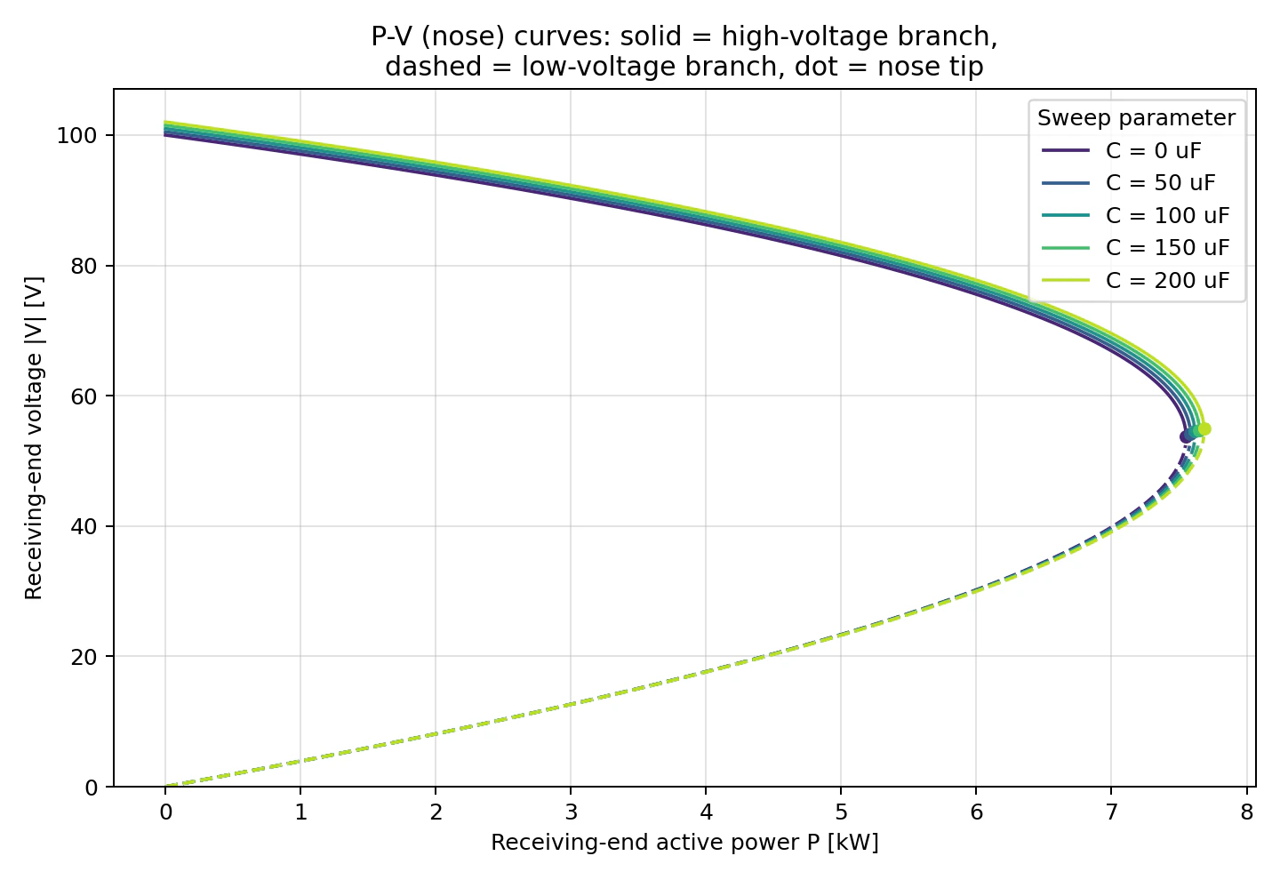
コンデンサ容量を増やすほど、受電端で無効電力の一部を局所的に補償できるため、同じ $P$ に対して電圧が高くなり、ノーズ先端もわずかに大きい $P$ 側へ移動する。ただし本記事の基準条件($L=1.0,\mathrm{mH}$, $\theta=30^\circ$)では、ノーズ先端付近の無効電力需要が数 kvar 程度であるのに対し、$C\le 200,\mu\mathrm F$ が供給できる無効電力 $Q_C=\omega C V^2$ はその一部にとどまるため、他の2枚の図と比べて曲線群の広がりは小さい。コンデンサの無効電力供給は $V^2$ に比例するため、電圧が下がるノーズ先端付近ほど補償効果自体も弱まる、という点も影響している。より大きな容量や、電圧一定型の無効電力補償(SVC など)と比較すると、この違いはさらに際立つはずである。
結果の読み方
- 高電圧枝(実線)では、$P$ の増加に対する電圧低下は比較的緩やかである。系統運用上、通常はこの枝の上で運転する。
- ノーズ先端で電圧安定余裕が尽き、これ以上の有効電力を定常的には供給できない。
- 低電圧枝(破線)は方程式上の解として存在するが、負荷の電圧・周波数特性や保護制御を考慮した実系統では、一般に不安定な運転点とみなされる。
- $X$ の低減、力率改善、受電端での無効電力補償は、いずれもノーズ先端を大きい $P$ 側へ押し上げる、すなわち電圧安定限界を改善する方向に働く。ただし本記事の設定では、コンデンサ容量の効果は他の2要因に比べて小さく現れており、効果の大きさは基準とする電圧・電力のスケールや負荷モデルに依存する。
まとめ
本記事では、無効電力とコンデンサの基礎的な回路モデル[1]を、P-V ノーズカーブの問題へ拡張した。受電端を PQ 負荷として扱い、電力バランス式から位相差 $\delta$ を代数的に消去することで、$V^2$ についての2次方程式という閉形式の関係式(4)を導いた。これにより、反復法を使わずに高電圧枝・低電圧枝の双方を一度に求められることを確認し、送電線リアクタンス・力率・コンデンサ容量を掃引した3種類の P-V 曲線群として可視化した。
次の発展としては、pu 法への正規化、変圧器タップ・分路リアクトルの追加、定インピーダンス/定電流/定電力を混在させた ZIP 負荷、そして式(4)の判別式を直接解いてノーズ先端の $P,V$ を陽に求める解析的な安定余裕評価を試したい。
参考文献
付録:実行用Pythonコード全文
次の内容を nose_curve.py として保存して実行すると、pv_l.png、pv_power_factor.png、pv_capacitance.png が同じフォルダに出力される。
"""Closed-form P-V (nose) curves for a two-bus system with a PQ load
and a shunt capacitor at the receiving end.

The receiving-end voltage V satisfies a quadratic equation in V^2 for
any given active power P, line impedance Z = R + jX (X = omega L),
load power factor angle theta, and capacitor susceptance omega*C.
Both roots of that quadratic are the classical high-voltage and
low-voltage branches of the nose curve; no iterative power-flow solver
is required.

Run:
    python nose_curve.py

It writes pv_l.png, pv_power_factor.png, and pv_capacitance.png.
"""

from pathlib import Path

import matplotlib.pyplot as plt
import numpy as np

OUTPUT_DIR = Path(__file__).parent
BASE = {
    "E": 100.0,
    "R": 0.10,
    "f": 50.0,
    "L": 1.0e-3,
    "theta": np.deg2rad(30.0),
    "C": 100e-6,
}
P_VALUES = np.linspace(1.0, 30_000.0, 4000)


def branch_voltages(P, E, R, L, f, theta, C):
    """Return (V_high, V_low) receiving-end voltages for each P.

    Derived from |E_dot - V_dot|/Z = I with S = P + jQ, Q = P tan(theta) -
    omega*C*V^2 (capacitor leading, load lagging positive). Squaring
    and summing the real/imaginary power-balance equations eliminates
    the unknown angle delta and leaves a quadratic in w = V^2:

        A w^2 + B(P) w + C_(P) = 0

    A does not depend on P; B is linear in P and C_ is quadratic in P,
    so for a fixed parameter set the discriminant B^2 - 4*A*C_ is
    itself a quadratic in P. Its zero is the nose tip.
    """
    omega = 2.0 * np.pi * f
    X = omega * L
    absZ = np.hypot(R, X)
    phi = np.arctan2(X, R)
    c1 = np.cos(phi) / absZ
    s1 = np.sin(phi) / absZ
    tan_th = np.tan(theta)
    k = omega * C

    A = c1 ** 2 + (s1 - k) ** 2
    B = 2.0 * P * (c1 + tan_th * (s1 - k)) - E ** 2 / absZ ** 2
    Cc = (P ** 2) * (1.0 + tan_th ** 2)

    disc = B ** 2 - 4.0 * A * Cc
    with np.errstate(invalid="ignore"):
        sqrt_disc = np.sqrt(np.where(disc >= 0.0, disc, np.nan))
        w_high = (-B + sqrt_disc) / (2.0 * A)
        w_low = (-B - sqrt_disc) / (2.0 * A)
        V_high = np.sqrt(np.where(w_high >= 0.0, w_high, np.nan))
        V_low = np.sqrt(np.where(w_low >= 0.0, w_low, np.nan))
    return V_high, V_low


def nose_tip(E, R, L, f, theta, C, p_max_search=200_000.0):
    """Locate the fold point (P, V) where the two branches merge."""
    P_fine = np.linspace(1.0, p_max_search, 400_000)
    V_high, V_low = branch_voltages(P_fine, E, R, L, f, theta, C)
    valid = np.isfinite(V_high)
    if not np.any(valid):
        return None
    idx = np.where(valid)[0][-1]
    return P_fine[idx], V_high[idx]


def plot_family(values, key, label, filename, base=BASE):
    """Overlay a family of nose curves (both branches) for a swept
    parameter, colour-coded by the swept value."""
    fig, ax = plt.subplots(figsize=(8, 5.5))
    colors = plt.get_cmap("viridis")(np.linspace(0.1, 0.9, len(values)))
    for value, color in zip(values, colors):
        params = {**base, key: value}
        V_high, V_low = branch_voltages(P_VALUES, **params)
        ax.plot(P_VALUES / 1000.0, V_high, color=color, label=label(value))
        ax.plot(P_VALUES / 1000.0, V_low, color=color, linestyle="--")
        tip = nose_tip(**params)
        if tip is not None:
            ax.plot(tip[0] / 1000.0, tip[1], "o", color=color, markersize=5,
                    zorder=5)
    ax.set_xlabel("Receiving-end active power P [kW]")
    ax.set_ylabel("Receiving-end voltage |V| [V]")
    ax.set_title("P-V (nose) curves: solid = high-voltage branch,\n"
                  "dashed = low-voltage branch, dot = nose tip")
    ax.set_ylim(bottom=0)
    ax.grid(True, alpha=0.35)
    ax.legend(title="Sweep parameter", loc="upper right")
    fig.tight_layout()
    fig.savefig(OUTPUT_DIR / filename, dpi=180)
    plt.close(fig)


def main():
    plot_family(
        [0.4e-3, 0.7e-3, 1.0e-3, 1.3e-3, 1.6e-3],
        "L", lambda L: f"L = {L * 1e3:.1f} mH", "pv_l.png")
    plot_family(
        np.deg2rad([10, 20, 30, 40, 50]),
        "theta", lambda theta: f"cos(theta) = {np.cos(theta):.2f}",
        "pv_power_factor.png")
    plot_family(
        [0, 50e-6, 100e-6, 150e-6, 200e-6],
        "C", lambda C: f"C = {C * 1e6:.0f} uF", "pv_capacitance.png")


if __name__ == "__main__":
    main()
実行には NumPy と Matplotlib が必要である。
pip install numpy matplotlib