『経済・ファイナンスデータの計量時系列分析』
の章末問題で「コンピュータを用いて」とあるものをRで解いています。

2.5
- (1)
library(forecast)

data<-read.table("economicdata.txt",header=T)
ar4<-Arima(diff(log(data$indprod))*100, order=c(4, 0, 0))
ma3<-Arima(diff(log(data$indprod))*100, order=c(0, 0, 3))
arma1_1<-Arima(diff(log(data$indprod))*100, order=c(1, 0, 1))
arma2_1<-Arima(diff(log(data$indprod))*100, order=c(2, 0, 1))
arma1_2<-Arima(diff(log(data$indprod))*100, order=c(1, 0, 2))
arma2_2<-Arima(diff(log(data$indprod))*100, order=c(2, 0, 2))

name<-c('AR(4)', 'MA(3)', 'ARMA(1,1)', 'ARMA(2,1)', 'ARMA(1,2)', 'ARMA(2,2)')
aic<-c(
  AIC(ar4)/length(data$indprod),
  AIC(ma3)/length(data$indprod),
  AIC(arma1_1)/length(data$indprod),
  AIC(arma2_1)/length(data$indprod),
  AIC(arma1_2)/length(data$indprod),
  AIC(arma2_2)/length(data$indprod)
)
bic<-c(
  BIC(ar4)/length(data$indprod),
  BIC(ma3)/length(data$indprod),
  BIC(arma1_1)/length(data$indprod),
  BIC(arma2_1)/length(data$indprod),
  BIC(arma1_2)/length(data$indprod),
  BIC(arma2_2)/length(data$indprod)
)
out<-data.frame(matrix(aic, nrow=1))
out<-rbind(out, bic)
colnames(out)<-name
rownames(out)<-c('AIC', 'SIC')
out
       AR(4)    MA(3) ARMA(1,1) ARMA(2,1) ARMA(1,2) ARMA(2,2)
AIC 3.232032 3.239599  3.324956  3.277746  3.233284  3.246579
SIC 3.296225 3.293094  3.367752  3.331241  3.286779  3.310772
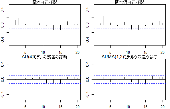
## figure
par(mfrow = c(2, 2))
par(mar = c(2, 2, 1, 1))
acf(diff(log(data$indprod)), xlim=c(1, 20), ylim=c(-0.5, 0.5))
mtext(text = '標本自己相関', side = 3)
pacf(diff(log(data$indprod)), xlim=c(1, 20), ylim=c(-0.5, 0.5))
mtext(text = '標本偏自己相関')
acf(ar4$residuals, xlim=c(1, 20), ylim=c(-0.5, 0.5))
mtext(text = 'AR(4)モデルの残差の診断', side = 3)
acf(arma1_2$residuals, xlim=c(1, 20), ylim=c(-0.5, 0.5))
mtext(text = 'ARMA(1,2)モデルの残差の診断', side = 3)
- (2)
library(forecast)

data<-read.table("economicdata.txt",header=T)
ar4<-Arima(diff(log(data$indprod))*100, order=c(4, 0, 0))
arma1_2<-Arima(diff(log(data$indprod))*100, order=c(1, 0, 2))
AR(4)
Box.test(ar4$residuals[1:10], type="Ljung")
	Box-Ljung test

data:  ar4$residuals[1:10]
X-squared = 0.37762, df = 1, p-value = 0.5389
p>0.05より帰無仮説を棄却できないので自己相関があるとは言えない。
ARMA(1, 2)
Box.test(arma1_2$residuals[1:10], type="Ljung")
	Box-Ljung test

data:  arma1_2$residuals[1:10]
X-squared = 0.37971, df = 1, p-value = 0.5378
p>0.05より帰無仮説を棄却できないので自己相関があるとは言えない。
2.6
library(forecast)
data<-read.table("arma.txt", header=T)
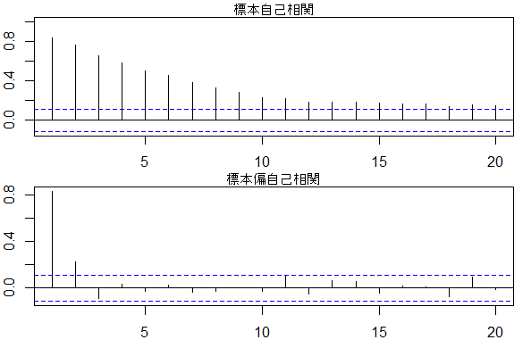
- (1)
par(mfrow=c(2, 1))
acf(data$y1, xlim=c(1, 20))
mtext('標本自己相関', side = 3)
pacf(data$y1, xlim=c(1, 20))
mtext('標本偏自己相関', side = 3)
- (2), (3)
###AR(2)
###ARMA(1,1),ARMA(2,1),ARMA(1,2),ARMA(2,2)
ar2<-Arima(data$y1, order=c(2, 0, 0))
arma1_1<-Arima(data$y1, order=c(1, 0, 1))
arma2_1<-Arima(data$y1, order=c(2, 0, 1))
arma1_2<-Arima(data$y1, order=c(1, 0, 2))
arma2_2<-Arima(data$y1, order=c(2, 0, 2))

name<-c('AR(2)', 'ARMA(1,1)', 'ARMA(2,1)', 'ARMA(1,2)', 'ARMA(2,2)')
aic<-c(
  AIC(ar2)/length(data$y1),
  AIC(arma1_1)/length(data$y1),
  AIC(arma2_1)/length(data$y1),
  AIC(arma1_2)/length(data$y1),
  AIC(arma2_2)/length(data$y1)
)
bic<-c(
  BIC(ar2)/length(data$y1),
  BIC(arma1_1)/length(data$y1),
  BIC(arma2_1)/length(data$y1),
  BIC(arma1_2)/length(data$y1),
  BIC(arma2_2)/length(data$y1)
)
out<-data.frame(matrix(aic, nrow=1))
out<-rbind(out, bic)
colnames(out)<-name
rownames(out)<-c('AIC', 'SIC')
###AIC ARMA(2,1), SIC AR(2)
out
       AR(2) ARMA(1,1) ARMA(2,1) ARMA(1,2) ARMA(2,2)
AIC 3.023947  3.034293  3.021437  3.029152  3.027627
SIC 3.073331  3.083677  3.083167  3.090882  3.101703
- (4)
AICからはARMA(2,1)、SICからはAR(2)を選択した。
acf(arma2_1$residuals, xlim=c(1,20), ylim=c(-0.5,0.5))
acf(ar2$residuals, xlim=c(1,20), ylim=c(-0.5,0.5))
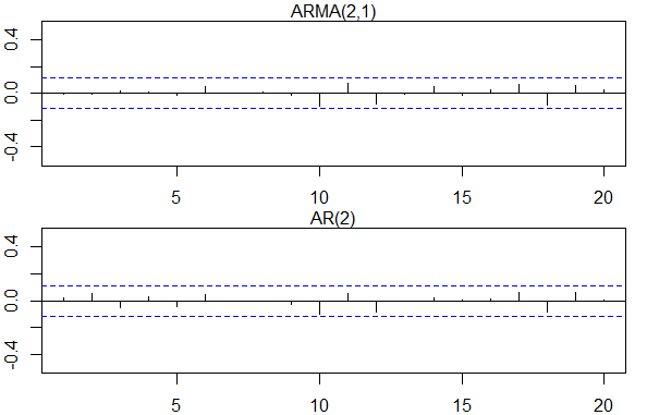
Box.test(arma2_1$residuals[1:20], type="Ljung")
	Box-Ljung test

data:  arma2_1$residuals[1:20]
X-squared = 0.013201, df = 1, p-value = 0.9085
Box.test(ar2$residuals[1:20], type="Ljung")
	Box-Ljung test

data:  ar2$residuals[1:20]
X-squared = 0.0979, df = 1, p-value = 0.7544
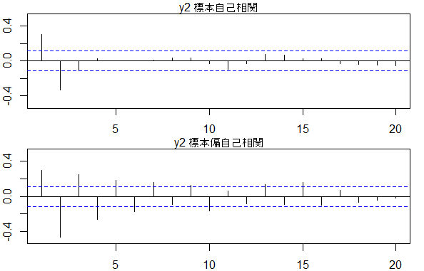
- (5)
y2
acf(data$y2, xlim = c(1, 20), ylim = c(-0.5, 0.5))
mtext(text = 'y2 標本自己相関', side = 3)
pacf(data$y2, xlim = c(1, 20), ylim = c(-0.5, 0.5))
mtext(text = 'y2 標本偏自己相関', side = 3)
####MA(3)
####ARMA(1,1),ARMA(2,1),ARMA(1,2),ARMA(2,2)
ma3<-Arima(data$y2, order=c(0, 0, 3))
arma1_1<-Arima(data$y2, order=c(1, 0, 1))
arma2_1<-Arima(data$y2, order=c(2, 0, 1))
arma1_2<-Arima(data$y2, order=c(1, 0, 2))
arma2_2<-Arima(data$y2, order=c(2, 0, 2))

name<-c('MA(3)', 'ARMA(1,1)', 'ARMA(2,1)', 'ARMA(1,2)', 'ARMA(2,2)')
aic<-c(
  AIC(ma3)/length(data$y2),
  AIC(arma1_1)/length(data$y2),
  AIC(arma2_1)/length(data$y2),
  AIC(arma1_2)/length(data$y2),
  AIC(arma2_2)/length(data$y2)
)
bic<-c(
  BIC(ma3)/length(data$y2),
  BIC(arma1_1)/length(data$y2),
  BIC(arma2_1)/length(data$y2),
  BIC(arma1_2)/length(data$y2),
  BIC(arma2_2)/length(data$y2)
)
out<-data.frame(matrix(aic, nrow=1))
out<-rbind(out, bic)
colnames(out)<-name
rownames(out)<-c('AIC', 'SIC')
###AIC MA(3), SIC MA(3)
out
       MA(3) ARMA(1,1) ARMA(2,1) ARMA(1,2) ARMA(2,2)
AIC 2.769046  2.859515  2.775498  2.818165  2.781784
SIC 2.830775  2.908899  2.837228  2.879895  2.855860
par(mfrow = c(1, 1))
acf(ma3$residuals, xlim=c(1,20), ylim=c(-0.5,0.5))
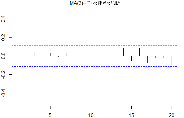
Box.test(ma3$residuals[1:20], type="Ljung")
	Box-Ljung test

data:  ma3$residuals[1:20]
X-squared = 0.0066437, df = 1, p-value = 0.935
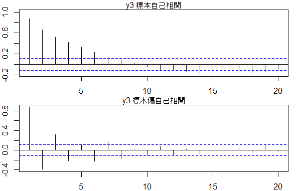
y3
###y3
par(mfrow=c(2,1))
acf(data$y3, xlim=c(1, 20))
mtext(text = 'y3 標本自己相関', side = 3)
pacf(data$y3, xlim=c(1, 20))
mtext(text = 'y3 標本偏自己相関', side = 3)
####AR(8), MA(7)
####ARMA(1,1),ARMA(2,1),ARMA(1,2),ARMA(2,2)
ar8<-Arima(data$y3, order=c(8, 0, 0))
ma7<-Arima(data$y3, order=c(0, 0, 7))
arma1_1<-Arima(data$y3, order=c(1, 0, 1))
arma2_1<-Arima(data$y3, order=c(2, 0, 1))
arma1_2<-Arima(data$y3, order=c(1, 0, 2))
arma2_2<-Arima(data$y3, order=c(2, 0, 2))

name<-c('AR(8)', 'MA(7)', 'ARMA(1,1)', 'ARMA(2,1)', 'ARMA(1,2)', 'ARMA(2,2)')
aic<-c(
  AIC(ar8)/length(data$y3),
  AIC(ma7)/length(data$y3),
  AIC(arma1_1)/length(data$y3),
  AIC(arma2_1)/length(data$y3),
  AIC(arma1_2)/length(data$y3),
  AIC(arma2_2)/length(data$y3)
)
bic<-c(
  BIC(ar8)/length(data$y3),
  BIC(ma7)/length(data$y3),
  BIC(arma1_1)/length(data$y3),
  BIC(arma2_1)/length(data$y3),
  BIC(arma1_2)/length(data$y3),
  BIC(arma2_2)/length(data$y3)
)
out<-data.frame(matrix(aic, nrow=1))
out<-rbind(out, bic)
colnames(out)<-name
rownames(out)<-c('AIC', 'SIC')
###AIC ARMA(1,2), SIC ARMA(1,1)
out
       AR(8)    MA(7) ARMA(1,1) ARMA(2,1) ARMA(1,2) ARMA(2,2)
AIC 3.115248 3.082550  3.069798   3.06590  3.065178  3.071635
SIC 3.238708 3.193663  3.119182   3.12763  3.126907  3.145711
par(mfrow = c(1, 1))
acf(arma1_2$residuals, xlim=c(1,20), ylim=c(-0.5,0.5))
mtext(text = 'ARMA(1,2)モデルの残差の診断', side = 3)
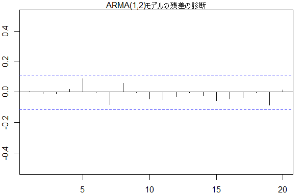
Box.test(arma1_2$residuals[1:20], type="Ljung")
	Box-Ljung test

data:  arma1_2$residuals[1:20]
X-squared = 0.17219, df = 1, p-value = 0.6782
acf(arma1_1$residuals, xlim=c(1,20), ylim=c(-0.5,0.5))
mtext(text = 'ARMA(1,1)モデルの残差の診断', side = 3)
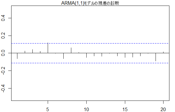
Box.test(arma1_1$residuals[1:20], type="Ljung")
	Box-Ljung test

data:  arma1_1$residuals[1:20]
X-squared = 6.0017e-05, df = 1, p-value = 0.9938
⇒ 3章はプログラムを用いる章末問題がないので、次は 『経済・ファイナンスデータの計量時系列分析』章末問題をRで解く-第4章VARモデル- へ