『経済・ファイナンスデータの計量時系列分析』
の章末問題で「コンピュータを用いて」とあるものをRで解いています。

Rで計量時系列分析:VARモデルから個々の時系列データ間の因果関係を推定するを参考にさせていただいた。
4.5
- (1) 表4.1
library(vars)
msci_day<-read.table("msci_day.txt",header=T)

# table4.1
msci_jp.p<-diff(log(msci_day$jp))*100
msci_uk.p<-diff(log(msci_day$uk))*100
msci_us.p<-diff(log(msci_day$us))*100

msci_jp_uk<-data.frame(cbind(msci_jp.p, msci_uk.p))
names(msci_jp_uk)<-c("jp", "uk")
VARselect(msci_jp_uk)
$selection
AIC(n)  HQ(n)  SC(n) FPE(n)
     3      1      1      3

$criteria
               1         2         3         4         5         6         7         8         9        10
AIC(n) 0.3902466 0.3875176 0.3874987 0.3925397 0.3900660 0.3906680 0.3946727 0.3977254 0.3958429 0.3983227
HQ(n)  0.3987528 0.4016947 0.4073466 0.4180584 0.4212555 0.4275283 0.4372038 0.4459273 0.4497157 0.4578663
SC(n)  0.4129850 0.4254150 0.4405550 0.4607550 0.4734402 0.4892012 0.5083648 0.5265765 0.5398529 0.5574917
FPE(n) 1.4773451 1.4733191 1.4732913 1.4807372 1.4770793 1.4779694 1.4839009 1.4884389 1.4856410 1.4893315
msci_jp_uk.var<-VAR(msci_jp_uk,p=3)
summary(msci_jp_uk.var)
VAR Estimation Results:
=========================
Endogenous variables: jp, uk
Deterministic variables: const
Sample size: 1387
Log Likelihood: -4191.851
Roots of the characteristic polynomial:
0.4821 0.3647 0.3647 0.3208 0.3208 0.2654
Call:
VAR(y = msci_jp_uk, p = 3)


Estimation results for equation jp:
===================================
jp = jp.l1 + uk.l1 + jp.l2 + uk.l2 + jp.l3 + uk.l3 + const

      Estimate Std. Error t value Pr(>|t|)
jp.l1 -0.13654    0.02786  -4.901 1.07e-06 ***
uk.l1  0.42950    0.03268  13.143  < 2e-16 ***
jp.l2 -0.07311    0.02804  -2.607  0.00923 **
uk.l2  0.09295    0.03529   2.634  0.00853 **
jp.l3 -0.03010    0.02611  -1.153  0.24911
uk.l3  0.04430    0.03470   1.277  0.20197
const  0.03042    0.03268   0.931  0.35218
---
Signif. codes:  0 ‘***’ 0.001 ‘**’ 0.01 ‘*’ 0.05 ‘.’ 0.1 ‘ ’ 1


Residual standard error: 1.213 on 1380 degrees of freedom
Multiple R-Squared: 0.117,	Adjusted R-squared: 0.1131
F-statistic: 30.46 on 6 and 1380 DF,  p-value: < 2.2e-16


Estimation results for equation uk:
===================================
uk = jp.l1 + uk.l1 + jp.l2 + uk.l2 + jp.l3 + uk.l3 + const

        Estimate Std. Error t value Pr(>|t|)
jp.l1 -0.0146396  0.0237612  -0.616 0.537923
uk.l1 -0.1005008  0.0278722  -3.606 0.000322 ***
jp.l2 -0.0092070  0.0239193  -0.385 0.700357
uk.l2  0.0573500  0.0301004   1.905 0.056950 .
jp.l3  0.0006251  0.0222692   0.028 0.977609
uk.l3 -0.0591019  0.0295968  -1.997 0.046032 *
const  0.0499850  0.0278742   1.793 0.073154 .
---
Signif. codes:  0 ‘***’ 0.001 ‘**’ 0.01 ‘*’ 0.05 ‘.’ 0.1 ‘ ’ 1


Residual standard error: 1.034 on 1380 degrees of freedom
Multiple R-Squared: 0.02038,	Adjusted R-squared: 0.01612
F-statistic: 4.784 on 6 and 1380 DF,  p-value: 7.721e-05


Covariance matrix of residuals:
       jp     uk
jp 1.4703 0.3345
uk 0.3345 1.0696

Correlation matrix of residuals:
       jp     uk
jp 1.0000 0.2668
uk 0.2668 1.0000
uk_jp.granger<-causality(msci_jp_uk.var,cause="uk")$Granger
jp_uk.granger<-causality(msci_jp_uk.var,cause="jp")$Granger

msci_jp_us<-data.frame(cbind(msci_jp.p, msci_us.p))
names(msci_jp_us)<-c("jp", "us")
VARselect(msci_jp_us)
$selection
AIC(n)  HQ(n)  SC(n) FPE(n)
     3      2      2      3

$criteria
                1            2            3            4            5            6            7            8           9          10
AIC(n) 0.01461004 -0.008767984 -0.009367858 -0.005606025 -0.003056226 -0.006456374 -0.003083306 -0.002622352 -0.00207798 0.001241809
HQ(n)  0.02311628  0.005409070  0.010480018  0.019912672  0.028133293  0.030403966  0.039447856  0.045579632  0.05179483 0.060785436
SC(n)  0.03734847  0.029129398  0.043688477  0.062609263  0.080318015  0.092076820  0.110608841  0.126228748  0.14193207 0.160410815
FPE(n) 1.01471731  0.991270405  0.990676056  0.994410027  0.996949113  0.993565531  0.996923149  0.997383570  0.99792765 1.001247285
msci_jp_us.var<-VAR(msci_jp_us,p=3)
summary(msci_jp_us.var)
VAR Estimation Results:
=========================
Endogenous variables: jp, us
Deterministic variables: const
Sample size: 1387
Log Likelihood: -3921.058
Roots of the characteristic polynomial:
0.3662 0.3662 0.3112 0.2847 0.2847 0.2166
Call:
VAR(y = msci_jp_us, p = 3)


Estimation results for equation jp:
===================================
jp = jp.l1 + us.l1 + jp.l2 + us.l2 + jp.l3 + us.l3 + const

      Estimate Std. Error t value Pr(>|t|)
jp.l1 -0.12668    0.02694  -4.703 2.82e-06 ***
us.l1  0.62892    0.03649  17.234  < 2e-16 ***
jp.l2 -0.08717    0.02671  -3.264  0.00113 **
us.l2  0.25234    0.04054   6.224 6.43e-10 ***
jp.l3 -0.03088    0.02433  -1.269  0.20457
us.l3  0.10262    0.04009   2.560  0.01058 *
const  0.02469    0.03132   0.788  0.43058
---
Signif. codes:  0 ‘***’ 0.001 ‘**’ 0.01 ‘*’ 0.05 ‘.’ 0.1 ‘ ’ 1


Residual standard error: 1.162 on 1380 degrees of freedom
Multiple R-Squared: 0.1885,	Adjusted R-squared: 0.185
F-statistic: 53.42 on 6 and 1380 DF,  p-value: < 2.2e-16


Estimation results for equation us:
===================================
us = jp.l1 + us.l1 + jp.l2 + us.l2 + jp.l3 + us.l3 + const

       Estimate Std. Error t value Pr(>|t|)
jp.l1  0.013212   0.019898   0.664    0.507
us.l1 -0.111843   0.026959  -4.149 3.55e-05 ***
jp.l2 -0.001773   0.019731  -0.090    0.928
us.l2 -0.031419   0.029951  -1.049    0.294
jp.l3  0.004470   0.017970   0.249    0.804
us.l3  0.008875   0.029616   0.300    0.764
const  0.033431   0.023135   1.445    0.149
---
Signif. codes:  0 ‘***’ 0.001 ‘**’ 0.01 ‘*’ 0.05 ‘.’ 0.1 ‘ ’ 1


Residual standard error: 0.8587 on 1380 degrees of freedom
Multiple R-Squared: 0.01275,	Adjusted R-squared: 0.00846
F-statistic: 2.971 on 6 and 1380 DF,  p-value: 0.006924


Covariance matrix of residuals:
       jp     us
jp 1.3512 0.0883
us 0.0883 0.7373

Correlation matrix of residuals:
        jp      us
jp 1.00000 0.08846
us 0.08846 1.00000
us_jp.granger<-causality(msci_jp_us.var,cause="us")$Granger
jp_us.granger<-causality(msci_jp_us.var,cause="jp")$Granger

msci_uk_us<-data.frame(cbind(msci_uk.p, msci_us.p))
names(msci_uk_us)<-c("uk", "us")
VARselect(msci_uk_us)
$selection
AIC(n)  HQ(n)  SC(n) FPE(n)
     3      2      2      3

$criteria
                1          2          3          4          5          6          7          8          9         10
AIC(n) -0.6108435 -0.6352794 -0.6374497 -0.6360516 -0.6355264 -0.6329052 -0.6315587 -0.6267474 -0.6221105 -0.6240250
HQ(n)  -0.6023373 -0.6211024 -0.6176018 -0.6105329 -0.6043369 -0.5960448 -0.5890276 -0.5785454 -0.5682377 -0.5644814
SC(n)  -0.5881051 -0.5973820 -0.5843933 -0.5678363 -0.5521522 -0.5343720 -0.5178666 -0.4978963 -0.4781004 -0.4648560
FPE(n)  0.5428927  0.5297875  0.5286390  0.5293787  0.5296569  0.5310474  0.5317632  0.5343283  0.5368122  0.5357861
msci_uk_us.var<-VAR(msci_uk_us,p=3)
summary(msci_uk_us.var)
VAR Estimation Results:
=========================
Endogenous variables: uk, us
Deterministic variables: const
Sample size: 1387
Log Likelihood: -3484.284
Roots of the characteristic polynomial:
0.4796 0.3646 0.3646 0.2949 0.2949 0.1073
Call:
VAR(y = msci_uk_us, p = 3)


Estimation results for equation uk:
===================================
uk = uk.l1 + us.l1 + uk.l2 + us.l2 + uk.l3 + us.l3 + const

      Estimate Std. Error t value Pr(>|t|)
uk.l1 -0.32624    0.03053 -10.687  < 2e-16 ***
us.l1  0.49923    0.03424  14.579  < 2e-16 ***
uk.l2 -0.04092    0.03164  -1.293  0.19612
us.l2  0.19095    0.03817   5.003 6.38e-07 ***
uk.l3 -0.08355    0.02833  -2.949  0.00324 **
us.l3  0.08628    0.03650   2.364  0.01823 *
const  0.03980    0.02593   1.535  0.12508
---
Signif. codes:  0 ‘***’ 0.001 ‘**’ 0.01 ‘*’ 0.05 ‘.’ 0.1 ‘ ’ 1


Residual standard error: 0.9624 on 1380 degrees of freedom
Multiple R-Squared: 0.1516,	Adjusted R-squared: 0.148
F-statistic: 41.11 on 6 and 1380 DF,  p-value: < 2.2e-16


Estimation results for equation us:
===================================
us = uk.l1 + us.l1 + uk.l2 + us.l2 + uk.l3 + us.l3 + const

        Estimate Std. Error t value Pr(>|t|)
uk.l1 -0.0005434  0.0272247  -0.020 0.984079
us.l1 -0.1095305  0.0305391  -3.587 0.000347 ***
uk.l2  0.0028284  0.0282209   0.100 0.920181
us.l2 -0.0249528  0.0340429  -0.733 0.463695
uk.l3 -0.0302226  0.0252635  -1.196 0.231787
us.l3  0.0240891  0.0325552   0.740 0.459460
const  0.0346515  0.0231299   1.498 0.134330
---
Signif. codes:  0 ‘***’ 0.001 ‘**’ 0.01 ‘*’ 0.05 ‘.’ 0.1 ‘ ’ 1


Residual standard error: 0.8583 on 1380 degrees of freedom
Multiple R-Squared: 0.01356,	Adjusted R-squared: 0.009271
F-statistic: 3.162 on 6 and 1380 DF,  p-value: 0.004393


Covariance matrix of residuals:
       uk     us
uk 0.9262 0.3948
us 0.3948 0.7367

Correlation matrix of residuals:
       uk     us
uk 1.0000 0.4779
us 0.4779 1.0000
uk_us.granger<-causality(msci_uk_us.var,cause="uk")$Granger
us_uk.granger<-causality(msci_uk_us.var,cause="us")$Granger

out<-data.frame(matrix(c(uk_jp.granger$statistic[1],
                         us_jp.granger$statistic[1],
                         jp_uk.granger$statistic[1],
                         us_uk.granger$statistic[1],
                         jp_us.granger$statistic[1],
                         uk_us.granger$statistic[1]),nrow=1))
out<-rbind(out, c(uk_jp.granger$p.value,
                  us_jp.granger$p.value,
                  jp_uk.granger$p.value,
                  us_uk.granger$p.value,
                  jp_us.granger$p.value,
                  uk_us.granger$p.value))
colnames(out)<-c("UK->JP", "US->JP", "JP->UK", "US->UK", "JP->US", "UK->US")
rownames(out)<-c("検定統計量","P値")
out
             UK->JP   US->JP    JP->UK   US->UK    JP->US    UK->US
検定統計量 58.79556 104.5269 0.1614905 71.36158 0.1720271 0.5486038
P値         0.00000   0.0000 0.9222796  0.00000 0.9153345 0.6490908
……、本のp83 表4.1と合わないですね、…… 誤り分かる方ご指摘下さい。
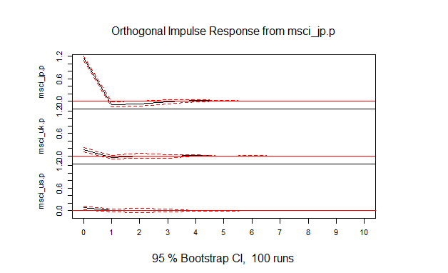
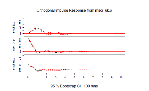
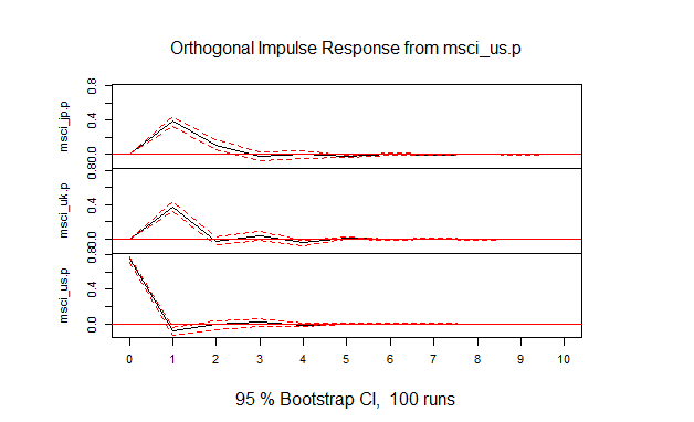
- (1) 図4.1
msci_jp_uk_us<-data.frame(cbind(msci_jp.p, msci_uk.p, msci_us.p))
VARselect(msci_jp_uk_us)
msci.var<-VAR(msci_jp_uk_us,p=3)
msci.irf<-irf(msci.var,ci=0.95)
plot(msci.irf)
JPに対するJP, UK, USの反応
UKに対するJP, UK, USの反応
USに対するJP, UK, USの反応
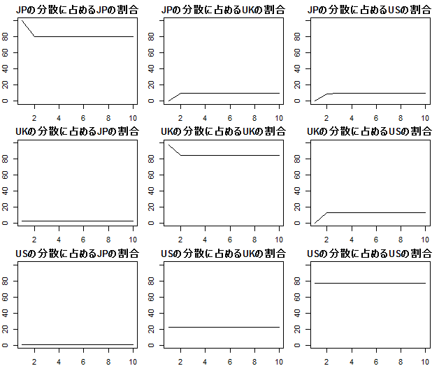
- (1) 図4.2
msci.fevd<-fevd(msci.var)
par(mfrow=c(3,3))
par(mar=c(2, 2, 2, 1))
plot(msci.fevd$msci_jp.p[,1]*100,type="l",ylim=c(0,100),ylab="",main="JPの分散に占めるJPの割合")
plot(msci.fevd$msci_jp.p[,2]*100,type="l",ylim=c(0,100),ylab="",main="JPの分散に占めるUKの割合")
plot(msci.fevd$msci_jp.p[,3]*100,type="l",ylim=c(0,100),ylab="",main="JPの分散に占めるUSの割合")
plot(msci.fevd$msci_uk.p[,1]*100,type="l",ylim=c(0,100),ylab="",main="UKの分散に占めるJPの割合")
plot(msci.fevd$msci_uk.p[,2]*100,type="l",ylim=c(0,100),ylab="",main="UKの分散に占めるUKの割合")
plot(msci.fevd$msci_uk.p[,3]*100,type="l",ylim=c(0,100),ylab="",main="UKの分散に占めるUSの割合")
plot(msci.fevd$msci_us.p[,1]*100,type="l",ylim=c(0,100),ylab="",main="USの分散に占めるJPの割合")
plot(msci.fevd$msci_us.p[,2]*100,type="l",ylim=c(0,100),ylab="",main="USの分散に占めるUKの割合")
plot(msci.fevd$msci_us.p[,3]*100,type="l",ylim=c(0,100),ylab="",main="USの分散に占めるUSの割合")
par(mfrow=c(1,1))
par(mar=c(3,3,3,3))
4.6
library(vars)
msci_day<-read.table("msci_day.txt",header=T)
- (1)
msci_jp.p<-diff(log(msci_day$jp))*100
msci_fr.p<-diff(log(msci_day$fr))*100
msci_ca.p<-diff(log(msci_day$ca))*100
-
(2)
jpの外生性が高く以下fr, ca
jp-uk-usと時差地理的にほぼ同等なので妥当 -
(3)
外生性が高い順 -
(4)
msci_jfc<-data.frame(cbind(msci_jp.p, msci_fr.p, msci_ca.p))
names(msci_jfc)<-c("jp", "fr", "ca")
VARselect(msci_jfc)
$selection
AIC(n)  HQ(n)  SC(n) FPE(n)
     2      1      1      2

$criteria
               1         2         3         4         5         6         7
AIC(n) 0.2412037 0.2348374 0.2372172 0.2464376 0.2460225 0.2505104 0.2553570
HQ(n)  0.2582161 0.2646092 0.2797483 0.3017281 0.3140723 0.3313196 0.3489256
SC(n)  0.2866805 0.3144219 0.3509093 0.3942374 0.4279299 0.4665255 0.5054798
FPE(n) 1.2727803 1.2647034 1.2677173 1.2794615 1.2789323 1.2846877 1.2909329
               8         9        10
AIC(n) 0.2619935 0.2659460 0.2719333
HQ(n)  0.3683214 0.3850333 0.4037799
SC(n)  0.5462239 0.5842841 0.6243790
FPE(n) 1.2995336 1.3046865 1.3125293
msci_jfc.var<-VAR(msci_jfc,p=2)
summary(msci_jfc.var)
VAR Estimation Results:
=========================
Endogenous variables: jp, fr, ca
Deterministic variables: const
Sample size: 1388
Log Likelihood: -6052.969
Roots of the characteristic polynomial:
0.3314 0.2705 0.2705 0.2349 0.2349 0.003481
Call:
VAR(y = msci_jfc, p = 2)


Estimation results for equation jp:
===================================
jp = jp.l1 + fr.l1 + ca.l1 + jp.l2 + fr.l2 + ca.l2 + const

      Estimate Std. Error t value Pr(>|t|)
jp.l1 -0.16613    0.02771  -5.995 2.60e-09 ***
fr.l1  0.30166    0.03394   8.887  < 2e-16 ***
ca.l1  0.25645    0.03651   7.024 3.37e-12 ***
jp.l2 -0.07788    0.02561  -3.042   0.0024 **
fr.l2  0.07928    0.03485   2.275   0.0231 *
ca.l2  0.01687    0.03733   0.452   0.6513
const  0.01088    0.03186   0.342   0.7328
---
Signif. codes:  0 ‘***’ 0.001 ‘**’ 0.01 ‘*’ 0.05 ‘.’ 0.1 ‘ ’ 1


Residual standard error: 1.179 on 1381 degrees of freedom
Multiple R-Squared: 0.1675,	Adjusted R-squared: 0.1639
F-statistic:  46.3 on 6 and 1381 DF,  p-value: < 2.2e-16


Estimation results for equation fr:
===================================
fr = jp.l1 + fr.l1 + ca.l1 + jp.l2 + fr.l2 + ca.l2 + const

      Estimate Std. Error t value Pr(>|t|)
jp.l1 -0.03864    0.02658  -1.454   0.1463
fr.l1 -0.15762    0.03256  -4.841 1.44e-06 ***
ca.l1  0.21916    0.03502   6.258 5.20e-10 ***
jp.l2 -0.06463    0.02456  -2.631   0.0086 **
fr.l2  0.03572    0.03343   1.068   0.2856
ca.l2  0.06986    0.03580   1.951   0.0512 .
const  0.04789    0.03056   1.567   0.1173
---
Signif. codes:  0 ‘***’ 0.001 ‘**’ 0.01 ‘*’ 0.05 ‘.’ 0.1 ‘ ’ 1


Residual standard error: 1.131 on 1381 degrees of freedom
Multiple R-Squared: 0.03785,	Adjusted R-squared: 0.03367
F-statistic: 9.054 on 6 and 1381 DF,  p-value: 9.944e-10


Estimation results for equation ca:
===================================
ca = jp.l1 + fr.l1 + ca.l1 + jp.l2 + fr.l2 + ca.l2 + const

      Estimate Std. Error t value Pr(>|t|)
jp.l1  0.01591    0.02434   0.654  0.51338
fr.l1 -0.01942    0.02981  -0.652  0.51482
ca.l1  0.05925    0.03206   1.848  0.06485 .
jp.l2 -0.04301    0.02249  -1.913  0.05600 .
fr.l2  0.06311    0.03061   2.062  0.03941 *
ca.l2 -0.02857    0.03278  -0.872  0.38363
const  0.08118    0.02798   2.902  0.00377 **
---
Signif. codes:  0 ‘***’ 0.001 ‘**’ 0.01 ‘*’ 0.05 ‘.’ 0.1 ‘ ’ 1


Residual standard error: 1.035 on 1381 degrees of freedom
Multiple R-Squared: 0.008891,	Adjusted R-squared: 0.004585
F-statistic: 2.065 on 6 and 1381 DF,  p-value: 0.05459


Covariance matrix of residuals:
       jp     fr     ca
jp 1.3890 0.3319 0.2132
fr 0.3319 1.2781 0.6383
ca 0.2132 0.6383 1.0714

Correlation matrix of residuals:
       jp     fr     ca
jp 1.0000 0.2491 0.1748
fr 0.2491 1.0000 0.5455
ca 0.1748 0.5455 1.0000
(5)
causality(msci_jfc.var,cause="fr")
$Granger

	Granger causality H0: fr do not Granger-cause jp ca

data:  VAR object msci_jfc.var
F-Test = 22.248, df1 = 4, df2 = 4143, p-value < 2.2e-16


$Instant

	H0: No instantaneous causality between: fr and jp ca

data:  VAR object msci_jfc.var
Chi-squared = 338.02, df = 2, p-value < 2.2e-16
p<2.2e-16でありフランスから日本、カナダへのGranger因果性が存在する。
- (6)
msci_jfc.irf<-irf(msci_jfc.var,impulse="fr", response="jp", ci=0.95)
plot(msci_jfc.irf)
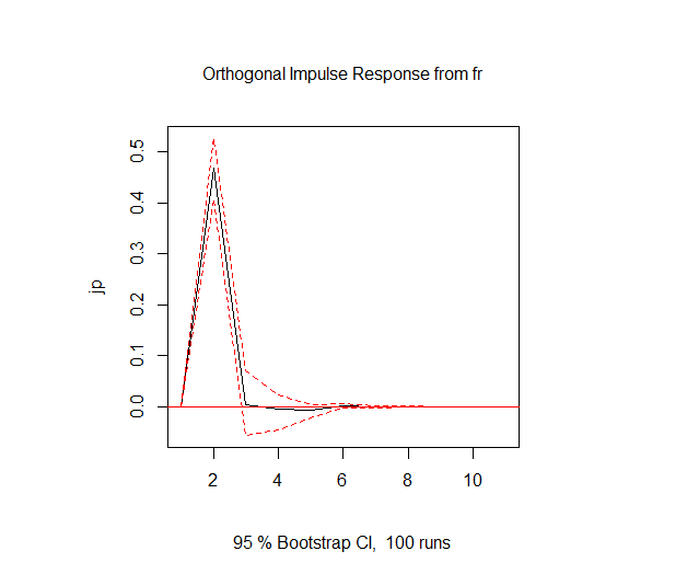
フランスにおける1標準偏差のショックは、1日後日本に0.45%程度のショックを与えるが2日以降ほぼショックはなくなる。
- (7)
msci_jfc.fevd<-fevd(msci_jfc.var)
par(mfrow=c(1,3))
plot(msci_jfc.fevd$ca[,1]*100,type="l",ylim=c(0,100),ylab="",main="CA-JP")
plot(msci_jfc.fevd$ca[,2]*100,type="l",ylim=c(0,100),ylab="",main="CA-FR")
plot(msci_jfc.fevd$ca[,3]*100,type="l",ylim=c(0,100),ylab="",main="CA-CA")
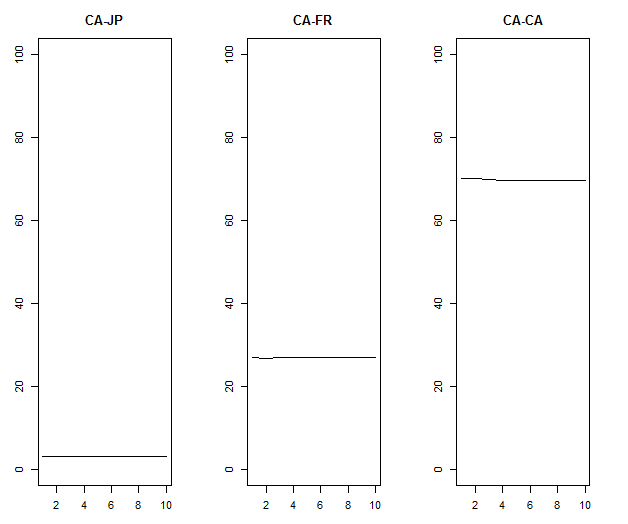
分散分析の結果は予測期間にほぼ依存しない。
予期できないカナダ市場の変動については日本市場が5%、フランス市場25%の説明力を持ち、70%はカナダ市場独自の要因で説明される。