stanアドカレ5日目の記事です。
昨日はkscscrさんの記事でした
ここまでで、stanの記法には慣れてきたのではないでしょうか。
私はstan歴3年目くらいですが、最初は何書いているのかちんぷんかんぷんでしたが、最近はちんぷん位になるには成長しました(?)
ある程度、数書いていればそのうち馴染んでくると思うので、頑張りぼんです。
はじめに
今日はロジスティック回帰モデルをやっていきます。
線形モデルは、データの生成に等分散正規分布を仮定しています。しかし、すべて正規分布とはいかんだろということで、線形モデルを他のデータに拡張(一般化)しようとなり、ロジスティック回帰などに発展していきます。
そういう意味で、線形モデルをいろんなタイプのデータに一般化したモデルのことを**一般化線形モデル(generalized linear model:GLM)**と呼びます。
なんで、他にも、ポアソン回帰もGLMに入ります。(線形モデルも等分散性正規分布を仮定したGLMと考えることもできます)。
では、ロジスティック回帰モデルは、どのようなデータに使うのか?
簡単に言うと、被説明変数が二値のデータ(0,1)であるときに使われます。二値データに用いることが出来るという汎用性の高さから、医学や社会科学など幅広い分野で用いられています。
- 生存か(1) or 死亡か(0)
- 心理的苦痛を抱えているか(1) or 心理的苦痛を抱えていないか(0)
- コンバージョンするか(1) or コンバージョンしないか(0)
線形モデルの様な正規分布を仮定すると、予測値として0~1以外の値が出てきてしまうので、($-\infty,+\infty$)の範囲をとりうる説明変数の線形結合を(0,1)の範囲に変換する必要があります。
変換には様々な方法があるらしい(俺知らない)のですが、変換のリンク関数にロジスティック関数(logitの逆関数)を用いて、範囲を(0,1)にする回帰をロジスティック回帰(logistic regression)といいます。
$$
F(x) = \frac{1}{1+e^{-x}}
$$
ロジスティック回帰モデル
データセットと変数の説明
今回は、{ggplot2}よりdiamondsのデータセットの一部を用いて、ダイアモンドの価格(diamonds$price)に影響している変数の効果を推定します。
ダイアモンドの価格(diamonds$price)は連続値ですが、今回はロジスティック回帰モデルに落とし込むため、価格の上位25%以上のダイアモンドに1,そうでないものに0を与え、価格上位25%のダイアモンドに影響しているだろう変数の効果を見ていきます。
ダイアモンドの価格(diamonds$price)のDensity plot(クリスマスカラー)
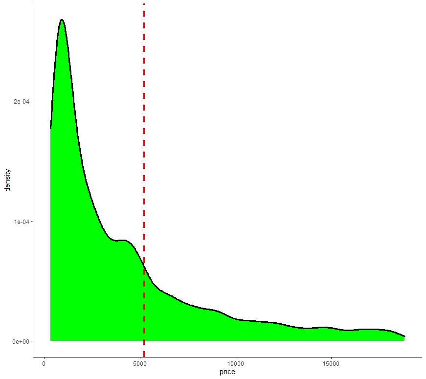
$5197を区切りに、$5197以上を1, $5197円未満に0を与えます。
今回は三つの説明変数を用いて、ダイアモンドの価格への効果を推定します。
-
carat : ダイアモンドの重さ
比率尺度:0.2 ~ 5.01
-
cut : カットの質
順序尺度:Fair, Good, Very Good, Premium, Ideal
-
clarity : ダイアモンドの明瞭度(透明度)
順序尺度:I1(最低),SI2,SI1,VS2,VS1,VVS2,VVS1,IF(最高)
モデル式
説明変数は3つありますのでモデルは以下の通りになります。
\begin{align}
q[n] =& {\rm inv\_logit}(\beta_0+\beta_1\times carat[n]+\beta_2\times cut[n]+\beta_3\times clarity[n])\\
Price[n]\sim& {\rm Bernoulli}(q[n])
\end{align}
- $n(1,N)$:データセットの行数(ダイアモンドデータの数)
- inv_logit():ロジスティック関数(ロジット関数の逆関数)
- Bernoulli():ベルヌーイ分布(ヤコブ・ベルヌーイに因んで名づけられた)
まず、三つの説明変数の線形結合をロジスティック関数を用いて0から1の範囲に変換します
\begin{align}
q[n] &= {\rm inv\_logit}(\beta_0+\beta_1\times carat[n]+\beta_2\times cut[n]+\beta_3\times clarity[n]) \\
&=\frac{1}{1+exp(-(\beta_0+\beta_1\times carat[n]+\beta_2\times cut[n]+\beta_3\times clarity[n]))}
\end{align}
つまり、
ダイアモンドの価格が上位25%か否か($price[n]$)は、パラメータ$q[n]$をもつベルヌーイ分布から生成される
という事になります。
Rとstanで推定
準備
# packages
# {tidyverse}が入っていない人はinstall.packages("tidyverse")
library(tidyverse)
library(rstan)
# {withr}が入っていない人はinstall.packages("withr")
library(withr) #乱数を固定するときに便利

# おまじない
options(mc.cores = parallel::detectCores())
rstan_options(auto_write = TRUE)

# 今回使うデータセット
diamonds

# A tibble: 53,940 x 10
   carat cut       color clarity depth table price     x     y     z
   <dbl> <ord>     <ord> <ord>   <dbl> <dbl> <int> <dbl> <dbl> <dbl>
 1 0.23  Ideal     E     SI2      61.5    55   326  3.95  3.98  2.43
 2 0.21  Premium   E     SI1      59.8    61   326  3.89  3.84  2.31
 3 0.23  Good      E     VS1      56.9    65   327  4.05  4.07  2.31
 4 0.290 Premium   I     VS2      62.4    58   334  4.2   4.23  2.63
 5 0.31  Good      J     SI2      63.3    58   335  4.34  4.35  2.75
 6 0.24  Very Good J     VVS2     62.8    57   336  3.94  3.96  2.48
 7 0.24  Very Good I     VVS1     62.3    57   336  3.95  3.98  2.47
 8 0.26  Very Good H     SI1      61.9    55   337  4.07  4.11  2.53
 9 0.22  Fair      E     VS2      65.1    61   337  3.87  3.78  2.49
10 0.23  Very Good H     VS1      59.4    61   338  4     4.05  2.39
# ... with 53,930 more rows
データの加工
diamonds_stan <-
  #seed値を42にして、diamondsデータセットから1%ランダムに抽出
  withr::with_seed(seed = 42, sample_frac(diamonds,size = 0.01)) %>%
  # 価格が$5197以上なら1,そうでなければ0
  mutate(price = if_else(price > 5197 ,1,0),
         # factor型の変数を数値型に変換
         across(where(is.factor), as.numeric))
-
diamondsは53940行あるデータなので、今回はデータのうちの1%(539要素)を使って推定していきます(重すぎるので。。。) -
diamonds$priceが$5197以上なら「1」,そうでなければ「0」を与える -
cut,clarityを順序に従って数値を振っていく
stanコード
data {
  int<lower=0> N; //データセットの要素数
  int<lower = 0, upper = 1>  price[N]; //ダイアモンドの価格
  real<lower=0> carat[N]; //ダイアモンドのカラット
  int<lower=0>  cut[N]; //ダイアモンドのカット
  int<lower=0>  clarity[N]; //ダイアモンドの明瞭度
}


parameters {
  real beta[4]; //今回推定するパラメータをベクトル型で渡す
  //以下でも可
  // real beta1;
  // real beta2;
  // real beta3;
  // real beta4;
}

transformed parameters{
  real q[N];
  for(n in 1:N){
    // 線形結合をロジスティック変換する
    q[n] = inv_logit(beta[1]+carat[n]*beta[2]+cut[n]*beta[3]+clarity[n]*beta[4]);
  }
}

model {
  for(n in 1:N){
    // ロジスティック変換したq[n]をパラメータにもつベルヌーイ分布から生成される
    price[n] ~ bernoulli(q[n]);
    //transformed_parametersブロックを使わずに以下でも可
    //price[n] ~ bernoulli_logit(beta[1]+carat[n]*beta[2]+cut[n]*beta[3]+clarity[n]*beta[4]);

  }
}

generated quantities{
  real pred_price[N];
  for(n in 1:N){
    // 推定されたパラメータを使ってダイアモンドの価格の予測を行う
    pred_price[n] = bernoulli_rng(q[n]);
  }
}
このコードをlogistic_reg.stanとして保存します(名前はなんでもいい)。
推定
# stan用にデータセットを生成
dataset <- list(price = diamonds_stan$price,
                carat = diamonds_stan$carat,
                cut = diamonds_stan$cut,
                clarity = diamonds_stan$clarity,
                N = nrow(diamonds_stan))

# stanで推定
fit <- stan(file = "logistic_reg.stan",  #ここは自分で作ったコードにしてね♬
            data = dataset,
            seed = 42,
            iter = 2000,
            warmup = 1000,
            chain = 4)
推定結果
# 推定結果のRhatがすべて1.10以下かを確認する関数(by dastatisさん)
>all(summary(fit)$summary[,'Rhat']<=1.10,na.rm = T)
[1] TRUE

>print(fit)
Inference for Stan model: logistic_reg.
4 chains, each with iter=2000; warmup=1000; thin=1;
post-warmup draws per chain=1000, total post-warmup draws=4000.

                  mean se_mean   sd   2.5%    25%    50%    75%  97.5% n_eff Rhat
beta[1]         -24.20    0.10 3.07 -30.57 -26.18 -24.05 -22.02 -18.73   983 1.01
beta[2]          16.27    0.06 2.11  12.53  14.76  16.18  17.61  20.74  1094 1.00
beta[3]           0.58    0.00 0.20   0.19   0.45   0.58   0.71   0.98  1659 1.00
beta[4]           1.28    0.01 0.21   0.89   1.13   1.27   1.41   1.70   983 1.01
q[1]              0.00    0.00 0.00   0.00   0.00   0.00   0.00   0.00  1877 1.00
q[2]              0.16    0.00 0.05   0.08   0.13   0.16   0.19   0.27  2079 1.00
q[3]              0.00    0.00 0.00   0.00   0.00   0.00   0.00   0.01  1553 1.00
- beta[1]:切片
- beta[2]:カラット
- beta[3]:カットの質
- beta[4]:明瞭度
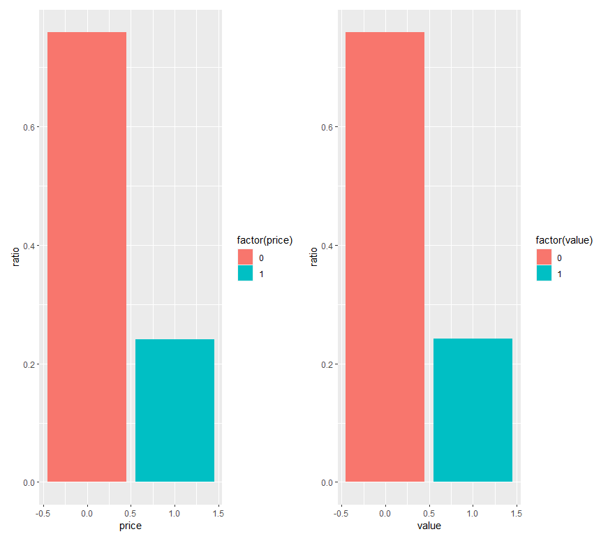
元データと事後予測分布の比較
# 元データのダイアモンドの価格(0,1)比率
row_plot <- diamonds_stan %>%
  count(price) %>%
  mutate(sum = sum(n),
         ratio = n/sum) %>%
  ggplot()+
  aes(x = price, y = ratio,fill=factor(price))+
  geom_bar(stat = "identity")


# ダイアモンドの価格の事後予測分布
fit_plot <- rstan::extract(fit,"pred_price") %>%
  as.data.frame() %>%
  as_tibble() %>%
  rowid_to_column("id") %>%
  pivot_longer(-id) %>%
  group_by(value) %>%
  count(value) %>%
  ungroup() %>%
  mutate(sum = sum(n),
         ratio = n/sum) %>%
  ggplot()+
  aes(x = value, y = ratio,fill = factor(value))+
  geom_bar(stat = "identity")

library(patchwork)
row_plot+fit_plot
左が元データ、右が事後予測分布
トレースプロット
stan_trace(fit,pars = "beta", separate_chains = T)
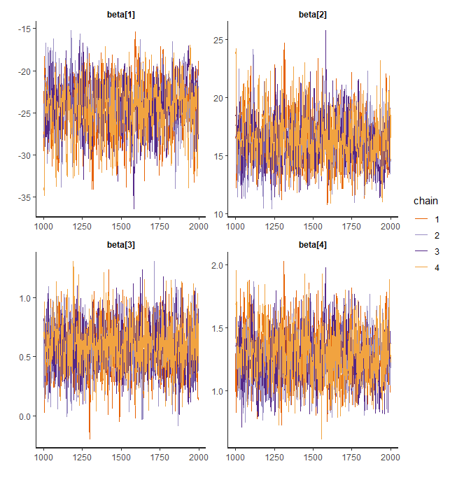
ゲジゲジみたいですね
デンシティプロット
stan_dens(fit,pars = "beta", separate_chains = T)
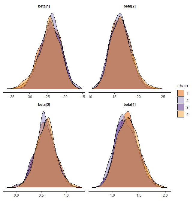
おおよそ、すべてのチェインで重なっているでしょう
おわりに
stanコードを書く上で重要なことは、データとモデルの対応関係がイメージできているかだと個人的には思います。
線形モデルでもGLMでも、これから先のブートキャンプで出てくるモデルにしても、モデルをグラフや数式として表現するのと同じように、stanの記法で表現するという意味で同じだと思います。この辺の能力はある程度慣れの部分が大きい(個人的に)と思うので、是非、ブートキャンプ続けてください!!
明日は、shu_ONさんの記事です
※{brms}つかうともっとみじかくかけるお
>library(brms)
>fit_brms <- brm(price ~ carat + cut + clarity, family = "bernoulli", data = diamonds_stan)
>fit_brms
Family: bernoulli
  Links: mu = logit
Formula: price ~ carat + cut + clarity
   Data: diamonds_stan (Number of observations: 539)
Samples: 4 chains, each with iter = 2000; warmup = 1000; thin = 1;
         total post-warmup samples = 4000

Population-Level Effects:
          Estimate Est.Error l-95% CI u-95% CI Rhat Bulk_ESS Tail_ESS
Intercept   -24.14      3.04   -30.45   -18.50 1.00     1332     1595
carat        16.25      2.09    12.48    20.47 1.00     1403     2076
cut           0.57      0.20     0.19     0.97 1.00     2388     2448
clarity       1.28      0.21     0.90     1.71 1.00     1663     2124

Samples were drawn using sampling(NUTS). For each parameter, Bulk_ESS
and Tail_ESS are effective sample size measures, and Rhat is the potential
scale reduction factor on split chains (at convergence, Rhat = 1).