目的
ゼロからKerasとTensorFlow(TF)を自由自在に動かせるようになる。
そのための、End to Endの作業ログ(備忘録)を残す。
※環境はMacだが、他のOSでの汎用性を保つように意識。
※アジャイルで執筆しており、精度を逐次高めていく予定。
環境
- Mac: 10.12.3
- Python: 3.6
- TensorFlow: 1.0.1
- Keras: 2.0.2
To Do
Keras導入編
Keras(Tensorflow)の環境構築<---いまココ
KerasでMINSTの学習と予測
KerasでTensorBoardの利用
Kerasで重みファイルの保存/読み込み
Kerasで自前データの学習と予測
Kerasで転移学習
流れ
Anacondaの仮想環境の中にTFとKerasをインストールし、サンプルコールを実行する。
Anacondaのインストールはpyenvを利用、Anacondaの公式サイトから直接インストールしても良い。
pyenvのインストール
git clone https://github.com/pyenv/pyenv.git ~/.pyenv
環境変数の設定 ※ターミナルを再起動すると設定が有効になる。
echo 'export PYENV_ROOT="$HOME/.pyenv"' >> ~/.bash_profile
echo 'export PATH="$PYENV_ROOT/bin:$PATH"' >> ~/.bash_profile
echo 'eval "$(pyenv init -)"' >> ~/.bash_profile
Anacondaのインストール
Anacondaのバージョン確認
pyenv install --list | grep anaconda3
以下が表示される。多くのバージョンが表示されるが、今回は末尾の部分のみ掲載した。
  anaconda3-4.2.0
  anaconda3-4.3.0
  anaconda3-4.3.1
最新版をインストール
// this will take time
pyenv install anaconda3-4.3.1
pyenv versions
pyenv global anaconda3-4.3.1
Anacondaの環境変数を設定 ※ターミナルを再起動すると設定が有効になる。
echo 'PATH="$PYENV_ROOT/versions/anaconda3-4.3.1/bin:$PATH"' >> ~/.bash_profile
Python 3.6の仮想環境の作成
py36という名前のPython3.6の仮想環境を作成する。
仮想環境のメリットは、例えばPython2系を使いたい場合に別の仮想環境を作れば、作業環境の切り分けが簡単になる。
// this will take time
conda create -n py36 python=3.6 anaconda
仮想環境を起動
source activate py36
作られた仮想環境の確認
conda info --envs
一覧が表示される。*は現在いる仮想環境
# conda environments:
#
py36                  *  /Users/XXX/anaconda/envs/py36
root                     /Users/XXX/anaconda
ちなみに、仮想環境を閉じたいときのコマンド
source deactivate py36
TFのインストール
pip install --ignore-installed --upgrade https://storage.googleapis.com/tensorflow/mac/cpu/tensorflow-1.0.1-py3-none-any.whl
pythonを立ち上げ稼働確認
python
以下を実行
import tensorflow as tf
hello = tf.constant('Hello, TensorFlow!')
sess = tf.Session()
print(sess.run(hello))
Hello, TensorFlow!が表示されたらセットアップ成功である。
python終了
quit()
Kerasのインストール
pip install keras==2.0.2
サンプルコードで挙動確認
Kerasのサンプルスクリプトのインストール
git clone https://github.com/fchollet/keras.git
グラフの表示に必要なライブラリのインストール
brewのインストールは公式サイトを参考:https://brew.sh/index_ja.html
// this will take time
brew install graphviz
pip install pydot
pip install pydot-ng
pip install graphviz
今回はMINSTを学習するサンプルを見てみる。Spyderというのはpythonの開発環境でAnacondaをインストールした時に付随する。
spyder keras/examples/mnist_mlp.py
実行時間短縮のためにepochs = 3にした。
また、後半にグラフ表示のためのスクリプトを追加した。
from __future__ import print_function
import keras
from keras.datasets import mnist
from keras.models import Sequential
from keras.layers import Dense, Dropout
from keras.optimizers import RMSprop
batch_size = 128
num_classes = 10
epochs = 3
# the data, shuffled and split between train and test sets
(x_train, y_train), (x_test, y_test) = mnist.load_data()
x_train = x_train.reshape(60000, 784)
x_test = x_test.reshape(10000, 784)
x_train = x_train.astype('float32')
x_test = x_test.astype('float32')
x_train /= 255
x_test /= 255
print(x_train.shape[0], 'train samples')
print(x_test.shape[0], 'test samples')
# convert class vectors to binary class matrices
y_train = keras.utils.to_categorical(y_train, num_classes)
y_test = keras.utils.to_categorical(y_test, num_classes)
model = Sequential()
model.add(Dense(512, activation='relu', input_shape=(784,)))
model.add(Dropout(0.2))
model.add(Dense(512, activation='relu'))
model.add(Dropout(0.2))
model.add(Dense(10, activation='softmax'))
model.summary()
model.compile(loss='categorical_crossentropy',
optimizer=RMSprop(),
metrics=['accuracy'])
history = model.fit(x_train, y_train,
batch_size=batch_size,
epochs=epochs,
verbose=1,
validation_data=(x_test, y_test))
score = model.evaluate(x_test, y_test, verbose=0)
print('Test loss:', score[0])
print('Test accuracy:', score[1])
### add to show graph
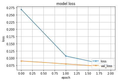
import matplotlib.pyplot as plt
def plot_history(history):
# print(history.history.keys())
# 精度の履歴をプロット
plt.plot(history.history['acc'], marker='.')
plt.plot(history.history['val_acc'], marker='.')
plt.title('model accuracy')
plt.xlabel('epoch')
plt.ylabel('accuracy')
plt.grid()
plt.legend(['acc', 'val_acc'], loc='lower right')
plt.show()
# 損失の履歴をプロット
plt.plot(history.history['loss'], marker='.')
plt.plot(history.history['val_loss'], marker='.')
plt.title('model loss')
plt.xlabel('epoch')
plt.ylabel('loss')
plt.grid()
plt.legend(['loss', 'val_loss'], loc='lower right')
plt.show()
plot_history(history)
Spyderの画面にある実行ボタン▶あまたはF5を押す、出力が表示される。
60000 train samples
10000 test samples
_________________________________________________________________
Layer (type)                 Output Shape              Param #
=================================================================
dense_10 (Dense)             (None, 512)               401920
_________________________________________________________________
dropout_7 (Dropout)          (None, 512)               0
_________________________________________________________________
dense_11 (Dense)             (None, 512)               262656
_________________________________________________________________
dropout_8 (Dropout)          (None, 512)               0
_________________________________________________________________
dense_12 (Dense)             (None, 10)                5130
=================================================================
Total params: 669,706.0
Trainable params: 669,706.0
Non-trainable params: 0.0
_________________________________________________________________
Train on 60000 samples, validate on 10000 samples
Epoch 1/3
60000/60000 [==============================] - 14s - loss: 0.2457 - acc: 0.9240 - val_loss: 0.1238 - val_acc: 0.9598
Epoch 2/3
60000/60000 [==============================] - 15s - loss: 0.1038 - acc: 0.9685 - val_loss: 0.0879 - val_acc: 0.9735
Epoch 3/3
60000/60000 [==============================] - 16s - loss: 0.0752 - acc: 0.9766 - val_loss: 0.0813 - val_acc: 0.9759
Test loss: 0.081280838731
Test accuracy: 0.9759
accとlossのグラフも表示される。

以上で環境構築は完了です。