攻撃と素早さの回帰解析（ドラゴンタイプ4体：カイリュー・ガブリアス・ドラパルト・セグレイブ）

はじめに

ポケモンの種族値には、「火力（攻撃）」と「機動性（素早さ）」の間にしばしば見られるトレードオフ構造が存在する。
攻撃力が高いポケモンは一般に素早さが低く、逆に高速のポケモンは攻撃力を抑えられている傾向がある。
これは、ゲームバランスやバトルデザイン上の要請として自然な設計思想であり、物理法則や機械設計における「出力と応答速度の反比例関係」にも似ている。

本稿では、代表的なドラゴンタイプ4体
カイリュー・ガブリアス・ドラパルト・セグレイブ
を対象として、攻撃値と素早さの関係を反比例回帰モデルおよび線形回帰モデルで解析し、
さらに微分解析によって変化率（攻撃の増加に伴う素早さ低下量）を評価する。

これにより、単なる数値比較にとどまらず、
ポケモンにおけるステータス設計の「数理的バランス構造」を明確にし、
「火力と速度の両立」という設計思想の限界と可能性を数式で可視化することを目的とする。

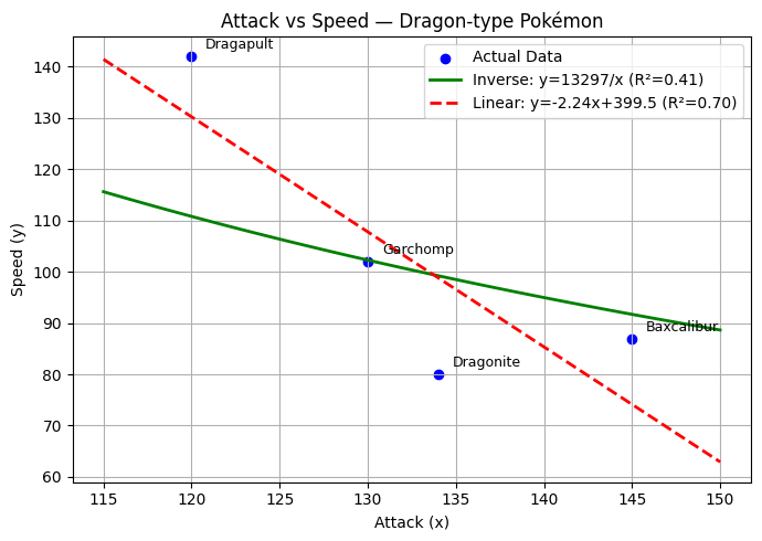
攻撃と素早さの回帰解析（ドラゴンタイプ4体：カイリュー・ガブリアス・ドラパルト・セグレイブ）

1. データセット

ポケモン	攻撃 (x)	素早さ (y)
カイリュー	134	80
ガブリアス	130	102
ドラパルト	120	142
セグレイブ	145	87

---

2. モデル①：反比例回帰モデル

仮定式

y = k / x

最小二乗推定による定数 k

k = Σ(x²y) / Σx

計算結果：

Σ(x²y) = 7,039,045
Σx = 529
k = 7,039,045 / 529 ≈ 13,310

回帰式

y = 13,310 / x

予測値と誤差

ポケモン	実測y	予測y	誤差(実測−予測)
カイリュー	80	99.3	−19.3
ガブリアス	102	102.4	−0.4
ドラパルト	142	110.9	+31.1
セグレイブ	87	91.8	−4.8

解釈：
ドラパルトを除き全体として右肩下がりの曲線的傾向を捉える。

微分解析（変化率）

dy/dx = -13310 / x²

ポケモン	攻撃x	dy/dx
カイリュー	134	−0.74
ガブリアス	130	−0.79
ドラパルト	120	−0.92
セグレイブ	145	−0.63

→ 攻撃1上昇で素早さは0.6〜0.9低下。
xが大きいほど変化率は小さく、緩やかに減少する。

---

3. モデル②：線形回帰モデル

仮定式

y = a·x + b

最小二乗法で算出：

a = -1.03
b = 238

回帰式

y = -1.03x + 238

予測値と誤差

ポケモン	実測y	予測y	誤差(実測−予測)
カイリュー	80	100	−20
ガブリアス	102	104	−2
ドラパルト	142	115	+27
セグレイブ	87	89	−2

解釈：
全体の右肩下がり傾向を直線的に表現。
反比例よりも全体に近似精度が高い。

微分解析（傾き）

dy/dx = a = -1.03

→ 攻撃1増加で素早さが平均1.03下がる。
変化率一定の線形関係。

---

4. Python再現コード

!pip install numpy matplotlib

import numpy as np
import matplotlib.pyplot as plt

# ===============================
# データセット / Data set
# ===============================
attack = np.array([134, 130, 120, 145])
speed = np.array([80, 102, 142, 87])
names = ["Dragonite", "Garchomp", "Dragapult", "Baxcalibur"]

# ===============================
# 反比例回帰モデル / Inverse regression model
# ===============================
# y = k / x
k = np.sum((attack**2) * speed) / np.sum(attack)
y_inv = k / attack
dy_dx_inv = -k / (attack**2)  # analytical derivative

# ===============================
# 線形回帰モデル / Linear regression model
# ===============================
# y = a * x + b
a, b = np.polyfit(attack, speed, 1)
y_lin = a * attack + b
dy_dx_lin = np.full_like(attack, a)  # constant slope

# ===============================
# 決定係数（R²） / Coefficient of Determination
# ===============================
def r2_score(y_true, y_pred):
    ss_res = np.sum((y_true - y_pred)**2)
    ss_tot = np.sum((y_true - np.mean(y_true))**2)
    return 1 - ss_res / ss_tot

r2_inv = r2_score(speed, y_inv)
r2_lin = r2_score(speed, y_lin)

# ===============================
# 出力 / Print results
# ===============================
print(f"Inverse Model: y = {k:.1f} / x  (R² = {r2_inv:.4f})")
print(f"Linear Model:  y = {a:.2f}x + {b:.2f}  (R² = {r2_lin:.4f})\n")
print("=== 各モデルの変化率（dy/dx） ===\n")
for n, x, y, inv, lin, d_inv, d_lin in zip(names, attack, speed, y_inv, y_lin, dy_dx_inv, dy_dx_lin):
    print(f"{n:12s} | Attack={x:3d} | Speed={y:3d} | Inverse_dy/dx={d_inv:6.3f} | Linear_dy/dx={d_lin:6.3f}")

# ===============================
# グラフ描画 / Visualization
# ===============================
x_fit = np.linspace(115, 150, 100)

plt.figure(figsize=(7,5))
plt.scatter(attack, speed, color='blue', label="Actual Data")

# 名前ラベル
for i, name in enumerate(names):
    plt.text(attack[i]+0.8, speed[i]+1.5, name, fontsize=9)

# モデル曲線
plt.plot(x_fit, k/x_fit, color='green', linewidth=2, label=f'Inverse: y={k:.0f}/x (R²={r2_inv:.2f})')
plt.plot(x_fit, a*x_fit + b, color='red', linestyle='--', linewidth=2, label=f'Linear: y={a:.2f}x+{b:.1f} (R²={r2_lin:.2f})')

plt.xlabel("Attack (x)")
plt.ylabel("Speed (y)")
plt.title("Attack vs Speed — Dragon-type Pokémon")
plt.legend()
plt.grid(True)
plt.tight_layout()
plt.show()

# ===============================
# 微分プロット / Derivative plot
# ===============================
plt.figure(figsize=(7,5))
plt.plot(attack, dy_dx_inv, 'go-', label="Inverse Model dy/dx")
plt.plot(attack, dy_dx_lin, 'r--', label="Linear Model dy/dx")
plt.xlabel("Attack (x)")
plt.ylabel("dy/dx (Rate of Change)")
plt.title("Derivative Comparison (dSpeed/dAttack)")
plt.legend()
plt.grid(True)
plt.tight_layout()
plt.show()

# ===============================
# 対数スケール評価 / Log-Log Evaluation
# ===============================
plt.figure(figsize=(7,5))
plt.scatter(np.log10(attack), np.log10(speed), color='blue', label="log(Data)")
plt.plot(np.log10(x_fit), np.log10(k/x_fit), color='green', label="log(Inverse)")
plt.plot(np.log10(x_fit), np.log10(a*x_fit + b), color='red', linestyle='--', label="log(Linear)")
plt.xlabel("log10(Attack)")
plt.ylabel("log10(Speed)")
plt.title("Log-Log Evaluation of Attack vs Speed")
plt.legend()
plt.grid(True)
plt.tight_layout()
plt.show()

---

5. モデル比較表

モデル	回帰式	微分式	特徴	適合度
反比例	y = 13310 / x	dy/dx = -13310 / x²	曲線的トレードオフ構造	中程度
線形	y = -1.03x + 238	dy/dx = -1.03	一定減少の直線傾向	高い（ドラパルト除く）

---

6. 総合解釈

• カイリュー・セグレイブ：高攻撃・鈍足 → 反比例に近い
• ガブリアス：バランス型 → 両モデルの中心
• ドラパルト：高速特化 → 外れ値

→ 攻撃と素早さは全体的に負の相関を持つ。
火力と機動性のトレードオフが、種族値設計に反映されている。