Transformerモデルとは
Transformerモデルとは、言葉や音、画像のように「順番のあるデータ(系列)」を理解し処理するためのAIの仕組みです。ChatGPTやBERTなど、現在の生成AIの多くはこのモデルの上に作られています。
昔のAI(RNNなど)は、文章を「1つずつ順番に」読んで理解していました。たとえば人間が左から右へ文章を読むように、先頭から少しずつ情報をため込みながら意味を推測していたのです。しかしこの方法では、文が長くなると前の情報を忘れたり、処理が遅くなったりするという弱点がありました。
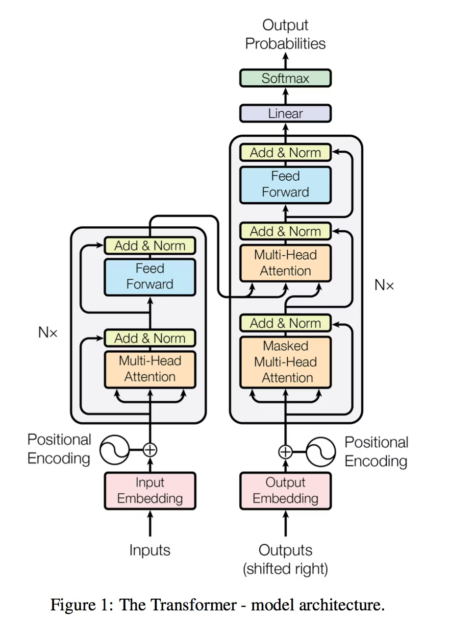
そこで登場したのがTransformerです。Transformerは、文の中のすべての単語を一度に見て、それぞれの単語が他のどの単語と関係しているかを数学的に計算します。この「関係の強さ」を求める仕組みを**Attention(注意機構)**と呼びます。たとえば「犬がボールを追いかけた」という文では、「犬」と「追いかけた」が深く結びついていることをAIが自動で見つけます。
Transformerの中では、単語が数のかたまり(ベクトル)として表され、ベクトル同士の内積をとることで意味の近さを測ります。そして指数関数や確率を使って、その関係を確率的に重み付けし、文全体の意味を平均化して理解します。次に来る単語を選ぶときも、確率の高いものを予測して文章を作ります。
1. 直線(Linear Function)
y = ax + b
→ ニューラルネットの基本単位
1層の出力:y = Wx + b
ここで W は重み行列。
直線が多次元化すると行列による「線形変換」となる。
Transformer の各層はこの線形写像(Affine transformation)を多数組み合わせた構造。
2. 連立方程式(Simultaneous Equations)
A·x = b
→ Attentionの重み計算や学習更新で現れる。
未知のベクトル x を求める過程は、ネットワークの内部で「入力と出力を結ぶ最適な係数」を解く操作と同じ。
最適化では常に Ax = b 型の関係(行列とベクトルの線形関係)を内包している。
3. 放物線(Quadratic Function)
y = ax² + bx + c
→ **損失関数(Loss Function)**の形。
学習では「誤差²」を最小化する。
L = (予測−正解)²
→ 微分して最小値を求める操作=誤差最小化。
放物線の最小点=AIが「最適な重み」を見つける点。
4. 指数関数(Exponential Function)
y = eˣ
→ Softmax関数や Attentionスコアで使用。
softmax(z_i) = exp(z_i) / Σ_j exp(z_j)
指数関数でスコアを滑らかに正の確率へ変換する。
指数は「成長率が自身に比例」という性質を持ち、情報の強調や拡散を数値的に制御できる。
5. 対数関数(Logarithm Function)
y = log(x)
→ 損失関数の対数尤度に使用。
Cross-Entropy Loss:
L = −Σ p(x) log q(x)
確率の差を評価するため、log関数で小さな確率の差を強調。
AIが「正解の確率を最大化」するように学習する基礎式。
6. 三角関数(Trigonometric Functions)
sinθ, cosθ
→ **Positional Encoding(位置情報)**に直結。
PE(pos, 2i) = sin(pos / 10000^(2i/d))
PE(pos, 2i+1) = cos(pos / 10000^(2i/d))
トランスフォーマーは単語の順番を三角関数の周期で表現する。
周期性=順序関係の数値的表現。
7. 微分(Differentiation)
dy/dx = lim(Δy/Δx)
→ **勾配降下法(Gradient Descent)**の核。
重み更新式:
W_new = W_old − η * ∂L/∂W
誤差関数Lの傾きを求め、下る方向に更新。
放物線の接線の傾きが「勾配」に相当する。
8. 積分(Integration)
∫ f(x) dx
→ 平均化・確率分布・Attentionの加重平均に対応。
Attention出力:
y = Σ softmax(QK^T) * V
これは離散的な積分(確率密度×値の積の和)。
積分が「重み付き平均」を求める操作であることと同じ。
正規分布の確率密度関数(PDF)
確率変数 X が平均 μ、分散 σ² の正規分布に従うとき、
確率密度関数は:
f(x) = (1 / √(2πσ²)) · exp( −(x−μ)² / (2σ²) )
この f(x) は「各点の確率密度」を表すが、
確率として意味を持つためには:
∫_{−∞}^{∞} f(x) dx = 1
が成り立たなければならない。
(全区間の確率の総和が1)
10. 複素数平面(Complex Plane)
複素数
z = a + bi
は、実部 a(現実の成分)と虚部 b(回転・位相の成分)をもつ数である。
これを平面上に表したものが複素数平面であり、
実軸(横軸)は「大きさ(振幅)」、虚軸(縦軸)は「位相(角度)」を表す。
AI、特に**トランスフォーマーモデル(Transformer)**の内部でも、
この複素数平面と同様の構造が働いている。
Transformerは「意味」や「関係性」を、数値的な回転・距離・角度として表現するモデルである。
1. 複素数とベクトル表現
Transformerでは、文章や音声、画像の情報をすべて
**ベクトル(数列)**として表す。
v = (x₁, x₂, ..., xₙ)
このベクトルは「意味空間上の点」であり、
複素数 a + bi と同様に**方向(角度)と大きさ(距離)**をもつ。
たとえば、
“king − man + woman ≈ queen”
という関係は、
ベクトル空間における回転と平行移動に相当する。
これは複素数の演算 z₁·e^{iθ} + c のように、
方向(意味)を回転させ、位置(文脈)をずらす操作と一致している。
Transformerはこれを多次元で行い、
「言葉の意味」や「文脈のずれ」を数学的に捉えている。
2. オイラーの公式とAttentionの回転
オイラーの公式:
e^{iθ} = cosθ + i sinθ
この式は、「複素数の回転」を表す。
Transformerの中心である Self-Attention(自己注意機構) は、
ベクトル空間での「意味的な回転・重み付け」に相当する。
Attentionの式:
Attention(Q, K, V) = softmax(QKᵀ / √d) · V
ここで、QKᵀ は「ベクトル間の内積」=「角度 cosθ」に対応する。
AIはこの角度をもとに「どの単語が他の単語に注目すべきか」を確率的に決める。
つまり、Attentionは複素数平面上での角度(相関)を確率分布に変換している。
トランスフォーマーは「文脈の回転行列」を学習しているといえる。
3. 位相と意味の時間構造
複素数の偏角 θ は、波の**位相(phase)**を表す。
Transformerでも、文の「順序」や「時間的ずれ」を扱うときに、
同じ数学的構造が使われている。
Transformerの**Positional Encoding(位置情報)**は次の式で定義される:
PE(pos, 2i) = sin(pos / 10000^{2i/d})
PE(pos, 2i+1) = cos(pos / 10000^{2i/d})
sin と cos の組み合わせは、
まさに e^{iθ} = cosθ + i sinθ の実部・虚部。
AIは、単語の「位置」を複素平面の**回転角(位相)**として符号化している。
これにより、文中の単語の前後関係を「時間の波」として捉え、
意味の順序を保持することができる。
4. FFTと異常検知
FFT(高速フーリエ変換)は、信号を複素数の回転成分に分解する手法。
時間軸上の信号 x(t) を複素平面上で回転ベクトルとして表すことで、
どの周波数(振動)が含まれているかを求める。
フーリエ変換:
X(f) = ∫ x(t) e^{−i2πft} dt
TransformerのAttentionも、
入力ベクトルを多方向に投影し「どの周波数(関係)」が重要かを学習する点で、
FFTと構造的に似ている。
また、異常検知においては、
通常の信号スペクトル(X_normal)と比較して
複素平面上での距離を測る:
‖X − X_normal‖² > 閾値 ⇒ 異常
つまり、Transformerが「文脈のずれ」を検出するのと同様、
FFTを使ったAIは「波形のずれ」を検出する。
どちらも複素空間上での回転・距離の変化を数学的に計測している。
!pip install numpy matplotlib --quiet
import numpy as np
import matplotlib.pyplot as plt
#──────────────────────────────────────────────────────────────────────────────
# Helper: Softmax
#──────────────────────────────────────────────────────────────────────────────
def softmax(z):
z = z - np.max(z)
ez = np.exp(z)
return ez / np.sum(ez)
#──────────────────────────────────────────────────────────────────────────────
# Helper: Positional Encoding
#──────────────────────────────────────────────────────────────────────────────
def positional_encoding(positions, d_model):
PE = np.zeros((positions, d_model))
for p in range(positions):
for i in range(0, d_model, 2):
denom = 10000 ** (2 * i / d_model)
PE[p, i] = np.sin(p / denom)
if i + 1 < d_model:
PE[p, i + 1] = np.cos(p / denom)
return PE
#──────────────────────────────────────────────────────────────────────────────
# Helper: LU Decomposition (Doolittle, no pivoting)
#──────────────────────────────────────────────────────────────────────────────
def lu_decompose(A):
n = A.shape[0]
L = np.zeros_like(A, dtype=float)
U = np.zeros_like(A, dtype=float)
for i in range(n):
for j in range(i, n):
U[i, j] = A[i, j] - np.sum(L[i, :i] * U[:i, j])
L[i, i] = 1.0
for j in range(i + 1, n):
if abs(U[i, i]) < 1e-12:
raise ZeroDivisionError("Zero pivot encountered; pivoting required.")
L[j, i] = (A[j, i] - np.sum(L[j, :i] * U[:i, i])) / U[i, i]
return L, U
def lu_solve(L, U, b):
n = L.shape[0]
y = np.zeros(n)
for i in range(n):
y[i] = b[i] - np.dot(L[i, :i], y[:i])
x = np.zeros(n)
for i in range(n - 1, -1, -1):
if abs(U[i, i]) < 1e-12:
raise ZeroDivisionError("Zero pivot encountered in U; pivoting required.")
x[i] = (y[i] - np.dot(U[i, i + 1:], x[i + 1:])) / U[i, i]
return x
#──────────────────────────────────────────────────────────────────────────────
# Data Preparation
#──────────────────────────────────────────────────────────────────────────────
# (1) Linear layer
x_lin = np.linspace(-2, 2, 200)
W, b = 1.5, 0.5
y_lin = W * x_lin + b
# (2) Softmax
z = np.linspace(-3, 3, 200)
p_soft = softmax(z)
# (3) Attention weights (toy)
np.random.seed(0)
Q = np.random.rand(4, 3)
K = np.random.rand(4, 3)
scores = (Q @ K.T) / np.sqrt(Q.shape[1])
W_attn = np.exp(scores)
W_attn = W_attn / np.sum(W_attn, axis=1, keepdims=True)
# (4) Positional Encoding
PE = positional_encoding(60, 8)
# (5) Complex rotation
theta = np.linspace(0, 2*np.pi, 400)
z_complex = np.exp(1j * theta)
# (6) Quadratic loss
xq = np.linspace(-3, 3, 200)
yq = xq**2
grad = 2 * xq
# (7) Linear system via LU
A = np.array([[2.0, 1.0],
[1.0, 2.0]])
b_vec = np.array([3.0, 1.0])
L, U = lu_decompose(A)
x_sol = lu_solve(L, U, b_vec)
x_vals = np.linspace(-2, 3, 400)
y_line1 = 3 - 2 * x_vals
y_line2 = (1 - x_vals) / 2.0
# (8) Gaussian Integration (Normal Distribution)
x_gauss = np.linspace(-5, 5, 400)
mu, sigma = 0, 1
f_gauss = (1 / np.sqrt(2 * np.pi * sigma**2)) * np.exp(- (x_gauss - mu)**2 / (2 * sigma**2))
area_gauss = np.trapz(f_gauss, x_gauss)
# (9) FFT
t = np.linspace(0, 1, 512, endpoint=False)
sig = np.sin(2*np.pi*5*t) + 0.5*np.sin(2*np.pi*15*t)
FFT = np.fft.fft(sig)
freq = np.fft.fftfreq(t.size, d=t[1]-t[0])
#──────────────────────────────────────────────────────────────────────────────
# Combined Figure
#──────────────────────────────────────────────────────────────────────────────
fig, axs = plt.subplots(3, 3, figsize=(15, 12))
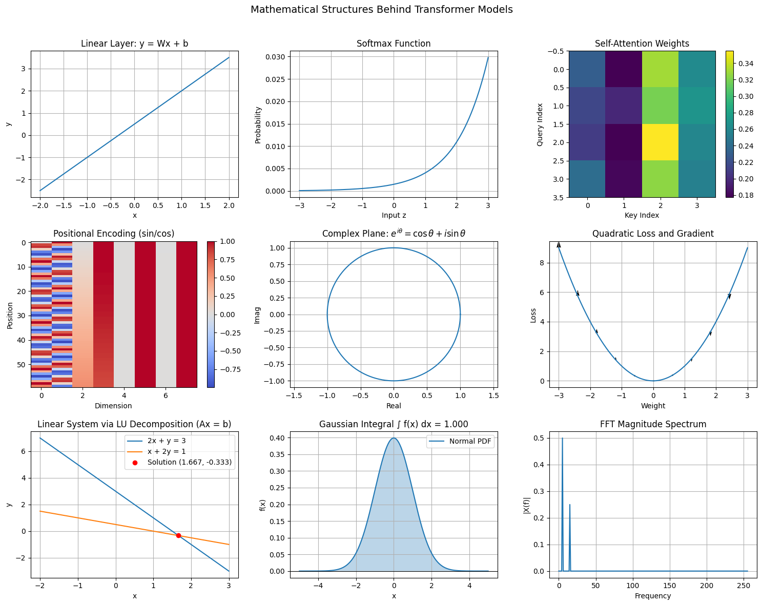
fig.suptitle("Mathematical Structures Behind Transformer Models", fontsize=14)
# (1) Linear layer
axs[0,0].plot(x_lin, y_lin)
axs[0,0].set_title("Linear Layer: y = Wx + b")
axs[0,0].set_xlabel("x")
axs[0,0].set_ylabel("y")
axs[0,0].grid(True)
# (2) Softmax
axs[0,1].plot(z, p_soft)
axs[0,1].set_title("Softmax Function")
axs[0,1].set_xlabel("Input z")
axs[0,1].set_ylabel("Probability")
axs[0,1].grid(True)
# (3) Attention heatmap
im0 = axs[0,2].imshow(W_attn, cmap="viridis")
axs[0,2].set_title("Self-Attention Weights")
axs[0,2].set_xlabel("Key Index")
axs[0,2].set_ylabel("Query Index")
fig.colorbar(im0, ax=axs[0,2])
# (4) Positional Encoding
im1 = axs[1,0].imshow(PE, aspect="auto", cmap="coolwarm")
axs[1,0].set_title("Positional Encoding (sin/cos)")
axs[1,0].set_xlabel("Dimension")
axs[1,0].set_ylabel("Position")
fig.colorbar(im1, ax=axs[1,0])
# (5) Complex rotation
axs[1,1].plot(np.real(z_complex), np.imag(z_complex))
axs[1,1].set_title("Complex Plane: $e^{i\\theta} = \\cos\\theta + i\\sin\\theta$")
axs[1,1].set_xlabel("Real")
axs[1,1].set_ylabel("Imag")
axs[1,1].axis("equal")
axs[1,1].grid(True)
# (6) Quadratic loss
axs[1,2].plot(xq, yq, label="y = x²")
axs[1,2].quiver(xq[::20], yq[::20], np.zeros_like(grad[::20]), -grad[::20],
angles='xy', scale_units='xy', scale=12, label="−∇y")
axs[1,2].set_title("Quadratic Loss and Gradient")
axs[1,2].set_xlabel("Weight")
axs[1,2].set_ylabel("Loss")
axs[1,2].grid(True)
# (7) Linear system via LU
axs[2,0].plot(x_vals, y_line1, label="2x + y = 3")
axs[2,0].plot(x_vals, y_line2, label="x + 2y = 1")
axs[2,0].plot(x_sol[0], x_sol[1], "ro", label=f"Solution ({x_sol[0]:.3f}, {x_sol[1]:.3f})")
axs[2,0].set_title("Linear System via LU Decomposition (Ax = b)")
axs[2,0].set_xlabel("x")
axs[2,0].set_ylabel("y")
axs[2,0].legend()
axs[2,0].grid(True)
# (8) Gaussian integral
axs[2,1].plot(x_gauss, f_gauss, label="Normal PDF")
axs[2,1].fill_between(x_gauss, 0, f_gauss, alpha=0.3)
axs[2,1].axhline(0, color="black", linewidth=0.8)
axs[2,1].set_title(f"Gaussian Integral ∫ f(x) dx = {area_gauss:.3f}")
axs[2,1].set_xlabel("x")
axs[2,1].set_ylabel("f(x)")
axs[2,1].legend()
axs[2,1].grid(True)
# (9) FFT
mask = freq >= 0
axs[2,2].plot(freq[mask], np.abs(FFT)[mask] / FFT.size)
axs[2,2].set_title("FFT Magnitude Spectrum")
axs[2,2].set_xlabel("Frequency")
axs[2,2].set_ylabel("|X(f)|")
axs[2,2].grid(True)
plt.tight_layout(rect=[0, 0, 1, 0.965])
plt.show()
# LU verification
print("A =\n", A)
print("L =\n", L)
print("U =\n", U)
print("Solution x =\n", x_sol)
print(f"Gaussian integral area = {area_gauss:.5f} (should ≈ 1.0)")