はじめに
この手法はまだ良い結果が得られていません.趣味としてアイデアを試している段階ですので,直ぐに使えるツールをお探しの方のお役には立てないと思います.ご了承下さい.m(__)m
[前回記事]DeepLearningとウェーブレット変換を用いた為替予測手法の検討
概要
今回やったことの概要を図1にまとめました.USD/JPYとEUR/JPYの5分足の終値を連続ウェーブレット変換して画像化し,AI(CNN)に学習させることで,12時間後の為替の動き(上がるor下がる)を予測できるか検討しました.学習回数=8000以上(これ以上学習回数を増やしても,学習データに対する正解率が上がらない)のテストデータに対する正解率の平均は53.7%でした.
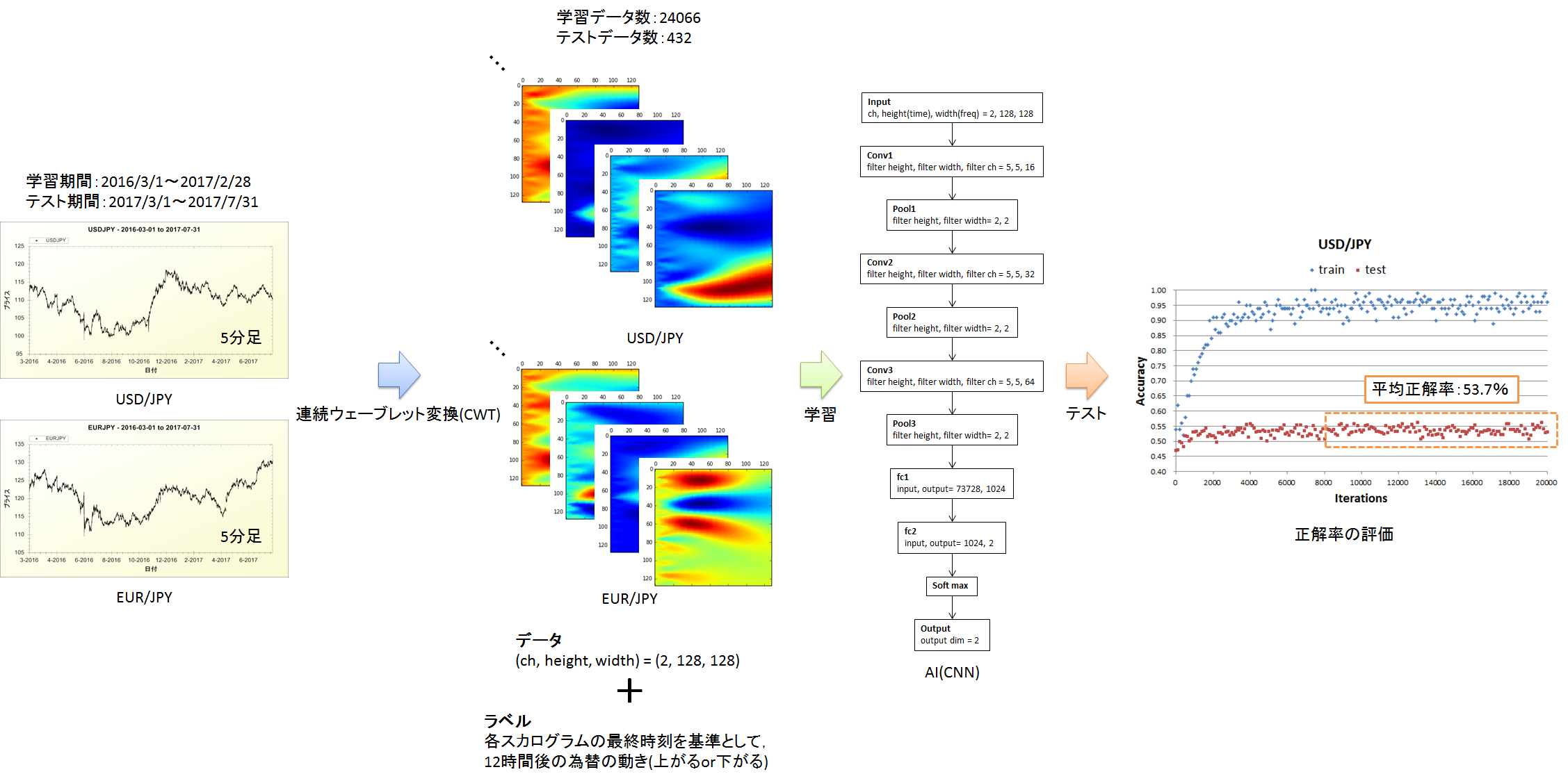
図1.今回やったことの概要
ウェーブレット変換とは
図2はウェーブレット変換の模式図を表しています.フーリエ変換は複雑な波形を無限に続く正弦波の足し合わせで表現する分析手法です.これに対してウェーブレット変換は局在波(ウェーブレット)の足し合わせで複雑な波形を表現します.フーリエ変換が定常的な信号の分析を得意とするのに対し,ウェーブレット変換は不規則,非定常な波形の解析に適しています.
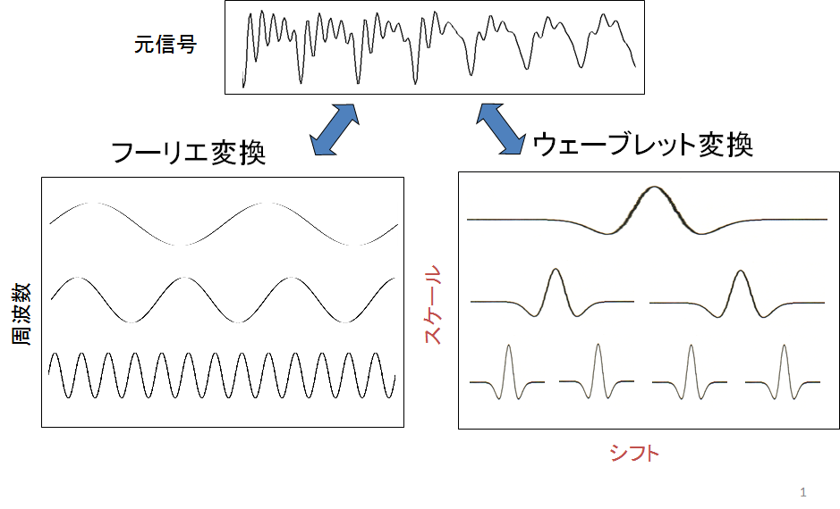
図2.ウェーブレット変換の模式図
出所:https://www.slideshare.net/ryosuketachibana12/ss-42388444
各シフト(時刻),各スケール(周波数)におけるウェーブレットの強さをマッピングしたものをスカログラムと呼びます.図2はy=sin(πx/16)のウェーブレット変換結果から作成したスカログラムです.このようにウェーブレット変換を用いることで任意の波形を画像化することが出来ます.
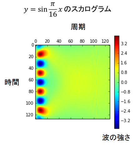
図3.スカログラムの例, y=sin(πx/16)
ウェーブレット変換には連続ウェーブレット変換(CWT)と離散ウェーブレット変換(DWT)がありますが,今回は連続ウェーブレット変換を使用しました.またウェーブレットには色々な形がありますが,とりあえずガウス関数を使用しています.
前回からの変更点
USD/JPYに加えてEUR/JPYを考慮する
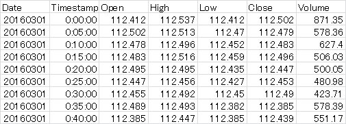
前回はUSD/JPYからUSD/JPYの値動きを予測しましたが,今回はUSD/JPYとEUR/JPYからUSD/JPYの値動きを予測します.USD/JPYとEUR/JPYそれぞれに対して同じ時刻のデータからスカログラム作成したいのですが,私が使用した為替データにはデータが欠損している時刻がありました.そのため,USD/JPYとEUR/JPYのどちらにも存在する時刻の為替データのみ抽出する必要がありました.そこで,以下のコードを作成しました.ちなみに私が使用した為替データは表1の様になっています.
表1.USD/JPY 5分足
import numpy as np

def align_USD_EUR(USD_csv, EUR_csv):
    """
    USD/JPYとEUR/JPYの欠損データを削除し,両者に存在する時刻の終値を抽出する関数
    USD_csv : USD/JPYの5分足のファイル名
    EUR_csv : EUR/JPYの5分足のファイル名
    """

    USD = np.loadtxt(USD_csv, delimiter = ",", usecols = (0,1,5), skiprows = 1, dtype="S8")
    EUR = np.loadtxt(EUR_csv, delimiter = ",", usecols = (0,1,5), skiprows = 1, dtype="S8")
    print("EUR shape " + str(EUR.shape)) # for debag
    print("USD shape " + str(USD.shape)) # for debag
    print("")

    USD_close = USD[:,2]
    EUR_close = EUR[:,2]
    USD = np.core.defchararray.add(USD[:,0], USD[:,1])
    EUR = np.core.defchararray.add(EUR[:,0], EUR[:,1])

    # 時刻が一致しないインデックス(idx_mismatch)を取得する
    if USD.shape[0] > EUR.shape[0]:

        temp_USD = USD[:EUR.shape[0]]
        coincidence = EUR == temp_USD
        idx_mismatch = np.where(coincidence == False)
        idx_mismatch = idx_mismatch[0][0]

    elif EUR.shape[0] > USD.shape[0]:

        temp_EUR = EUR[:USD.shape[0]]
        coincidence = USD == temp_EUR
        idx_mismatch = np.where(coincidence == False)
        idx_mismatch = idx_mismatch[0][0]

    elif USD.shape[0] == EUR.shape[0]:

        coincidence = USD == EUR
        idx_mismatch = np.where(coincidence == False)
        idx_mismatch = idx_mismatch[0][0]

    while USD.shape[0] != idx_mismatch:

        print("idx mismatch " + str(idx_mismatch)) # for debag
        print("USD[idx_mismatch] " + str(USD[idx_mismatch]))
        print("EUR[idx_mismatch] " + str(EUR[idx_mismatch]))

        # 不要なデータの削除
        if USD[idx_mismatch] > EUR[idx_mismatch]:
            EUR = np.delete(EUR, idx_mismatch)
            EUR_close = np.delete(EUR_close, idx_mismatch)
        elif EUR[idx_mismatch] > USD[idx_mismatch]:
            USD = np.delete(USD, idx_mismatch)
            USD_close = np.delete(USD_close, idx_mismatch)

        print("EUR shape " + str(EUR.shape)) # for debag
        print("USD shape " + str(USD.shape)) # for debag
        print("")

        if USD.shape[0] > EUR.shape[0]:

            temp_USD = USD[:EUR.shape[0]]
            coincidence = EUR == temp_USD
            idx_mismatch = np.where(coincidence == False)
            idx_mismatch = idx_mismatch[0][0]

        elif EUR.shape[0] > USD.shape[0]:

            temp_EUR = EUR[:USD.shape[0]]
            coincidence = USD == temp_EUR
            idx_mismatch = np.where(coincidence == False)
            idx_mismatch = idx_mismatch[0][0]

        elif USD.shape[0] == EUR.shape[0]:

            coincidence = USD == EUR
            if (coincidence==False).any():
                idx_mismatch = np.where(coincidence == False)
                idx_mismatch = idx_mismatch[0][0]
            else:
                idx_mismatch = np.where(coincidence == True)
                idx_mismatch = idx_mismatch[0].shape[0]

    USD = np.reshape(USD, (-1,1))
    EUR = np.reshape(EUR, (-1,1))
    USD_close = np.reshape(USD_close, (-1,1))
    EUR_close = np.reshape(EUR_close, (-1,1))

    USD = np.append(USD, EUR, axis=1)
    USD = np.append(USD, USD_close, axis=1)
    USD = np.append(USD, EUR_close, axis=1)
    np.savetxt("USD_EUR.csv", USD, delimiter = ",", fmt="%s")

    return USD_close, EUR_close
様々な期間のデータからスカログラムを作成する
前回はどのスカログラムも1日の波形データから作成しました.でも実際にトレードしている人たちは,評価する波形の期間を必要に応じて変化させています.そこで今回は異なる期間のデータからスカログラムを作成しました.データの期間は以下の様に選択しました.データ期間をもっと細かくすることは可能ですが,メモリの制約があってこれが限界でした.
学習データ:1日,1.5日,2日,2.5日,3日
テストデータ:1日
さて,ここで問題になるのが,データの期間を変えるとスカログラムのサイズが変わってしまうことです.CNNは異なるサイズの画像を学習することができません.そこで,画像処理ライブラリ「Pillow」を使って画像サイズを128x128に統一しました.
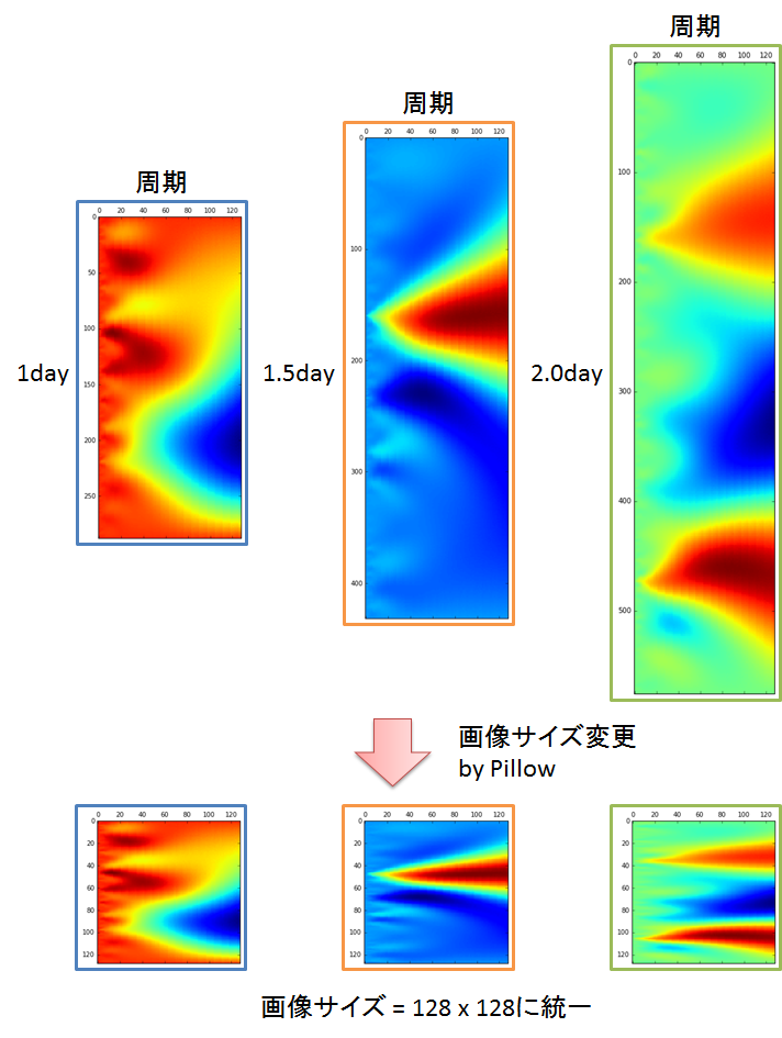
図4.画像サイズの統一の模式図
from PIL import Image
"""
original_scalogram : 元のスカログラム(numpy配列)
width              : サイズ変更後の画像の幅(=128)
height             : サイズ変更後の画像の高さ(=128)
"""
img_scalogram = Image.fromarray(original_scalogram)   # imageオブジェクトに変換
img_scalogram = img_scalogram.resize((width, height)) # 画像サイズ変更
array_scalogram = np.array(img_scalogram)             # numpy配列に変換
CNNの構造と学習フロー
CNNの構造と学習フローはそれぞれ図5,図6になります.
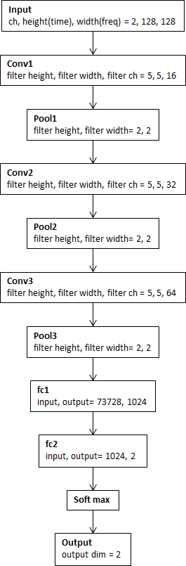
図5.CNNの構造
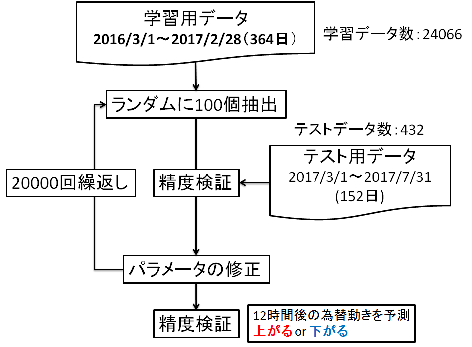
図6.学習フロー
計算結果
図7は学習データとテストデータに対する正解率の推移を示しています.学習回数=8000以上では学習データに対する正解率が上がらなくなります.学習回数=8000~20000のテストデータに対する正解率の平均は53.7%でした.学習回数=0~4000にてテストデータの正解率が上がっている様にも見えますが,ちょっと何とも言えない感じです.
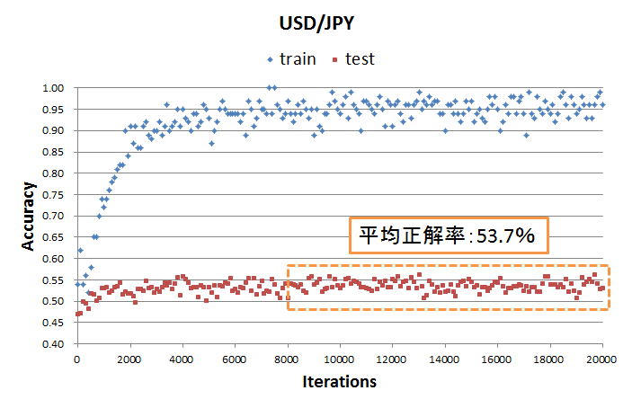
図7.正解率の推移
AIの予測結果は「上がる:82%,下がる:18%」の様に確率で出力されます.図8はテストデータに対する予測結果の推移を示しています.学習初期はほとんどのデータに対して確信度が低く,例えば「上がる:52%,下がる:48%」みたいな感じです.ところが,学習回数が増えるにつれて90%~100%ばかりになります.こんなに自信持って答えているのに,正解率=53.7%は違和感があります.
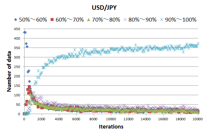
図8.テストデータに対する予測結果の推移
終わりに
という訳で,正解率>50%になったものの,偶然なのか,特徴がつかめているのか,まだまだ何とも言えない結果です...学習期間とテスト期間を変化させても同等の正解率が出るのか,検証する必要があると思います.
図8が示す様に,学習が進むにつれて確信度が高い予測結果が増えるという事は,学習データの中にテストデータと特徴が似ているスカログラムが含まれているという事です.正解率が上がらないのは,AIが似ていると判断したスカログラムでも,将来の値動きは学習データとテストデータで一致していないからだと思います.そこでユーロだけでなく他の通貨や金融データも考慮する(データのチャンネルを増やす)ことで,スカログラムが多様化し,上記の様なミスジャッジを減らせるかもなぁ,という希望を抱いています.とりあえず,正解率と比較して確信度が高い予測結果が多すぎますよね...笑
Yu-Nie
Appendix
分析に使ったデータは以下からダウンロードできます.
USDJPY_20160301_20170228_5min.csv
USDJPY_20170301_20170731_5min.csv
EURJPY_20160301_20170228_5min.csv
EURJPY_20170301_20170731_5min.csv
以下は分析に使ったコードです.
# 20170731
# y.izumi

import tensorflow as tf
import numpy as np
import scalogram4 as sca # FFTとスペクトログラム作成を行うためのモジュール
import time

"""パラメータの初期化と畳み込み演算,pooling演算を行う関数"""
# =============================================================================================================================================
# 重みの初期化関数
def weight_variable(shape, stddev=5e-3): # default stddev = 1e-4
    initial = tf.truncated_normal(shape, stddev=stddev)
    return tf.Variable(initial)
# バイアスの初期化関数
def bias_variable(shape):
    initial = tf.constant(0.0, shape=shape)
    return tf.Variable(initial)
# 畳み込み演算
def conv2d(x, W):
    return tf.nn.conv2d(x, W, strides=[1, 1, 1, 1], padding="SAME")
# pooling
def max_pool_2x2(x):
    return tf.nn.max_pool(x, ksize=[1, 2, 2, 1], strides=[1, 2, 2, 1], padding="SAME")
# =============================================================================================================================================

"""スカログラムの作成条件"""
# =============================================================================================================================================
train_USD_csv = "USDJPY_20160301_20170228_5min.csv"   # 為替データのファイル名, train
train_EUR_csv = "EURJPY_20160301_20170228_5min.csv"
# train_USD_csv = "USDJPY_20170301_20170731_5min.csv"   # 為替データのファイル名, train, for debag
# train_EUR_csv = "EURJPY_20170301_20170731_5min.csv"
test_USD_csv = "USDJPY_20170301_20170731_5min.csv"    # 為替データのファイル名, test
test_EUR_csv = "EURJPY_20170301_20170731_5min.csv"
# scales = np.arange(1,129)
predict_time_inc = 144                          # 値動きを予測する時刻の増分
# train_heights = [288]                         # スカログラムの高さ, num of time lines, リストで指定する
# test_heights = [288]
train_heights = [288, 432, 576, 720, 864]       # スカログラムの高さ, num of time lines, リストで指定する
test_heights = [288]
base_height = 128                               # 学習データに使用するスカログラムの高さ
width = 128                                     # スカログラムの幅,  num of freq lines
ch_flag = 1                                     # 四本値と出来高から使用するデータを選択する, ch_flag=1:close, 工事中(ch_flag=2:close and volume, ch_flag=5:start, high, low, close, volume)
input_dim = (ch_flag, base_height, width)       # channel = (1, 2, 5), height(time_lines), width(freq_lines)
save_flag = 0                                   # save_flag=1 : CWT係数をcsvファイルとして保存する, save_flag=0 : CWT係数をcsvファイルとして保存しない
scales = np.linspace(0.2,80,width)              # 使用するスケールをnumpy配列で指定する, スケールは分析に使用するウェーブレットの周波数に相当する, scalesが大きいと低周波, 小さいと高周波になる
wavelet = "gaus1"                               # ウェーブレットの名前, 'gaus1', 'gaus2', 'gaus3', 'gaus4', 'gaus5', 'gaus6', 'gaus7', 'gaus8', 'mexh'
tr_over_lap_inc = 4                             # CWT開始時刻の増分 train data
te_over_lap_inc = 36                            # CWT開始時刻の増分 test data
# ==============================================================================================================================================

"""スカログラムとラベルの作成"""
# ==============================================================================================================================================
# carry out CWT and make labels
print("Making the train data.")
x_train, t_train, freq = sca.merge_scalogram3(train_USD_csv, train_EUR_csv, scales, wavelet, train_heights, base_height, width, predict_time_inc, ch_flag, save_flag, tr_over_lap_inc)
# x_train, t_train, freq = sca.merge_scalogram3(test_USD_csv, test_EUR_csv, scales, wavelet, train_heights, base_height, width, predict_time_inc, ch_flag, save_flag, tr_over_lap_inc) # for debag

print("Making the test data.")
x_test, t_test, freq = sca.merge_scalogram3(test_USD_csv, test_EUR_csv, scales, wavelet, test_heights, base_height, width, predict_time_inc, ch_flag, save_flag, te_over_lap_inc)

# save scalograms and labels
print("Save scalogarams and labels")
np.savetxt(r"temp_result\x_train.csv", x_train.reshape(-1, 2*base_height*width), delimiter = ",")
np.savetxt(r"temp_result\x_test.csv", x_test.reshape(-1, 2*base_height*width), delimiter = ",")
np.savetxt(r"temp_result\t_train.csv", t_train, delimiter = ",", fmt = "%.0f")
np.savetxt(r"temp_result\t_test.csv", t_test, delimiter = ",", fmt = "%.0f")
np.savetxt(r"temp_result\frequency.csv", freq, delimiter = ",")

# load scalograms and labels
# print("Load scalogarams and labels")
# x_train = np.loadtxt(r"temp_result\x_train.csv", delimiter = ",")
# x_test = np.loadtxt(r"temp_result\x_test.csv", delimiter = ",")
# t_train = np.loadtxt(r"temp_result\t_train.csv", delimiter = ",", dtype = "i8")
# t_test = np.loadtxt(r"temp_result\t_test.csv", delimiter = ",", dtype = "i8")
# x_train = x_train.reshape(-1, 2, base_height, width)
# x_test = x_test.reshape(-1, 2, base_height, width)
# freq = np.loadtxt(r"temp_result\frequency.csv", delimiter = ",")

print("x_train shape " + str(x_train.shape))
print("t_train shape " + str(t_train.shape))
print("x_test shape " + str(x_test.shape))
print("t_test shape " + str(t_test.shape))
print("mean_t_train " + str(np.mean(t_train)))
print("mean_t_test " + str(np.mean(t_test)))
print("frequency " + str(freq))

# ==============================================================================================================================================

"""データ形状の加工"""
# ==============================================================================================================================================
# tensorflow用に次元を入れ替える
x_train = x_train.transpose(0, 2, 3, 1) # (num_data, ch, height(time_lines), width(freq_lines)) ⇒ (num_data, height(time_lines), width(freq_lines), ch)
x_test = x_test.transpose(0, 2, 3, 1)

train_size = x_train.shape[0]   # 学習データ数
test_size = x_test.shape[0]     # テストデータ数
train_batch_size = 100          # 学習バッチサイズ
test_batch_size = 600           # テストバッチサイズ

# labes to one-hot
t_train_onehot = np.zeros((train_size, 2))
t_test_onehot = np.zeros((test_size, 2))
t_train_onehot[np.arange(train_size), t_train] = 1
t_test_onehot[np.arange(test_size), t_test] = 1
t_train = t_train_onehot
t_test = t_test_onehot

# print("t train shape onehot" + str(t_train.shape)) # for debag
# print("t test shape onehot" + str(t_test.shape))
# ==============================================================================================================================================

"""CNNの構築"""
# ==============================================================================================================================================
x  = tf.placeholder(tf.float32, [None, input_dim[1], input_dim[2], 2]) # (num_data, height(time), width(freq_lines), ch), chは入力データのチャンネル数, USD/JPY, EUR/JPY ⇒ ch = 2
y_ = tf.placeholder(tf.float32, [None, 2]) # (num_data, num_label)
print("input shape ", str(x.get_shape()))

with tf.variable_scope("conv1") as scope:
    W_conv1 = weight_variable([5, 5, 2, 16])
    b_conv1 = bias_variable([16])
    h_conv1 = tf.nn.relu(conv2d(x, W_conv1) + b_conv1)
    h_pool1 = max_pool_2x2(h_conv1)
    print("conv1 shape ", str(h_pool1.get_shape()))

with tf.variable_scope("conv2") as scope:
    W_conv2 = weight_variable([5, 5, 16, 32])
    b_conv2 = bias_variable([32])
    h_conv2 = tf.nn.relu(conv2d(h_pool1, W_conv2) + b_conv2)
    h_pool2 = max_pool_2x2(h_conv2)
    print("conv2 shape ", str(h_pool2.get_shape()))
    h_pool2_height = int(h_pool2.get_shape()[1])
    h_pool2_width = int(h_pool2.get_shape()[2])

with tf.variable_scope("conv3") as scope:
    W_conv3 = weight_variable([5, 5, 32, 64])
    b_conv3 = bias_variable([64])
    h_conv3 = tf.nn.relu(conv2d(h_pool2, W_conv3) + b_conv3)
    h_pool3 = max_pool_2x2(h_conv3)
    print("conv3 shape ", str(h_pool3.get_shape()))
    h_pool3_height = int(h_pool3.get_shape()[1])
    h_pool3_width = int(h_pool3.get_shape()[2])

with tf.variable_scope("fc1") as scope:
    W_fc1 = weight_variable([h_pool3_height*h_pool3_width*64, 1024])
    b_fc1 = bias_variable([1024])
    h_pool3_flat = tf.reshape(h_pool3, [-1, h_pool3_height*h_pool3_width*64])
    h_fc1 = tf.nn.relu(tf.matmul(h_pool3_flat, W_fc1) + b_fc1)
    print("fc1 shape ", str(h_fc1.get_shape()))
    keep_prob = tf.placeholder(tf.float32)
    h_fc1_drop = tf.nn.dropout(h_fc1, keep_prob)

with tf.variable_scope("fc2") as scope:
    W_fc2 = weight_variable([1024, 2])
    b_fc2 = bias_variable([2])
    y_conv = tf.nn.softmax(tf.matmul(h_fc1_drop, W_fc2) + b_fc2)
    print("output shape ", str(y_conv.get_shape()))

# パラメータをtensorboardで可視化する
W_conv1 = tf.summary.histogram("W_conv1", W_conv1)
b_conv1 = tf.summary.histogram("b_conv1", b_conv1)
W_conv2 = tf.summary.histogram("W_conv2", W_conv2)
b_conv2 = tf.summary.histogram("b_conv2", b_conv2)
W_conv3 = tf.summary.histogram("W_conv3", W_conv3)
b_conv3 = tf.summary.histogram("b_conv3", b_conv3)
W_fc1 = tf.summary.histogram("W_fc1", W_fc1)
b_fc1 = tf.summary.histogram("b_fc1", b_fc1)
W_fc2 = tf.summary.histogram("W_fc2", W_fc2)
b_fc2 = tf.summary.histogram("b_fc2", b_fc2)
# ==============================================================================================================================================

"""誤差関数の指定"""
# ==============================================================================================================================================
# cross_entropy = -tf.reduce_sum(y_ * tf.log(y_conv))
cross_entropy = tf.reduce_sum(tf.nn.softmax_cross_entropy_with_logits(labels = y_, logits = y_conv))
loss_summary = tf.summary.scalar("loss", cross_entropy) # for tensorboard
# ==============================================================================================================================================

"""optimizerの指定"""
# ==============================================================================================================================================
optimizer = tf.train.AdamOptimizer(1e-4)
train_step = optimizer.minimize(cross_entropy)

# 勾配をtensorboardで可視化する
grads = optimizer.compute_gradients(cross_entropy)
dW_conv1 = tf.summary.histogram("dW_conv1", grads[0]) # for tensorboard
db_conv1 = tf.summary.histogram("db_conv1", grads[1])
dW_conv2 = tf.summary.histogram("dW_conv2", grads[2])
db_conv2 = tf.summary.histogram("db_conv2", grads[3])
dW_conv3 = tf.summary.histogram("dW_conv3", grads[4])
db_conv3 = tf.summary.histogram("db_conv3", grads[5])
dW_fc1 = tf.summary.histogram("dW_fc1", grads[6])
db_fc1 = tf.summary.histogram("db_fc1", grads[7])
dW_fc2 = tf.summary.histogram("dW_fc2", grads[8])
db_fc2 = tf.summary.histogram("db_fc2", grads[9])

# for i in range(8): # for debag
#     print(grads[i])
# ==============================================================================================================================================

"""精度検証用パラメータ"""
# ==============================================================================================================================================
correct_prediction = tf.equal(tf.argmax(y_conv,1), tf.argmax(y_,1))
accuracy = tf.reduce_mean(tf.cast(correct_prediction, tf.float32))
accuracy_summary = tf.summary.scalar("accuracy", accuracy) # for tensorboard
# ==============================================================================================================================================

"""学習の実行"""
# ==============================================================================================================================================
acc_list = []            # 正解率と誤差の途中経過を保存するリスト
num_data_each_conf = []  # 各確信度のデータ数の途中経過を保存するリスト
acc_each_conf = []       # 各確信度の正解率の途中経過を保存するリスト
start_time = time.time() # 計算時間のカウント
total_cal_time = 0

with tf.Session() as sess:
    saver = tf.train.Saver()
    sess.run(tf.global_variables_initializer())

    # tensorboard用ファイルの書き出し
    merged = tf.summary.merge_all()
    writer = tf.summary.FileWriter(r"temp_result", sess.graph)

    for step in range(20001):
        batch_mask = np.random.choice(train_size, train_batch_size)
        tr_batch_xs = x_train[batch_mask]
        tr_batch_ys = t_train[batch_mask]

        # 学習途中の精度確認
        if step%100 == 0:

            cal_time = time.time() - start_time # 計算時間のカウント
            total_cal_time += cal_time

            # train
            train_accuracy = accuracy.eval(feed_dict={x: tr_batch_xs, y_: tr_batch_ys, keep_prob: 1.0})
            train_loss = cross_entropy.eval(feed_dict={x: tr_batch_xs, y_: tr_batch_ys, keep_prob: 1.0})

            # test
            # use all data
            test_accuracy = accuracy.eval(feed_dict={x: x_test, y_: t_test, keep_prob: 1.0})
            test_loss = cross_entropy.eval(feed_dict={x: x_test, y_: t_test, keep_prob: 1.0})

            # use test batch
            # batch_mask = np.random.choice(test_size, test_batch_size, replace=False)
            # te_batch_xs = x_test[batch_mask]
            # te_batch_ys = t_test[batch_mask]
            # test_accuracy = accuracy.eval(feed_dict={x: te_batch_xs, y_: te_batch_ys, keep_prob: 1.0})
            # test_loss = cross_entropy.eval(feed_dict={x: te_batch_xs, y_: te_batch_ys, keep_prob: 1.0})

            print("calculation time %d sec, step %d, training accuracy %g, training loss %g, test accuracy %g, test loss %g"%(cal_time, step, train_accuracy, train_loss, test_accuracy, test_loss))
            acc_list.append([step, train_accuracy, test_accuracy, train_loss, test_loss])

            AI_prediction = y_conv.eval(feed_dict={x: x_test, y_: t_test, keep_prob: 1.0}) # AIの予測結果 use all data
            # AI_prediction = y_conv.eval(feed_dict={x: te_batch_xs, y_: te_batch_ys, keep_prob: 1.0}) # AIの予測結果 use test batch

            # print("AI_prediction.shape " + str(AI_prediction.shape)) # for debag
            # print("AI_prediction.type" + str(type(AI_prediction)))

            AI_correct_prediction = correct_prediction.eval(feed_dict={x: x_test, y_: t_test, keep_prob: 1.0}) # 正解:TRUE, 不正解:FALSE use all data
            # AI_correct_prediction = correct_prediction.eval(feed_dict={x: te_batch_xs, y_: te_batch_ys, keep_prob: 1.0}) # 正解:TRUE, 不正解:FALSE use test batch

            # print("AI_prediction.shape " + str(AI_prediction.shape)) # for debag
            # print("AI_prediction.type" + str(type(AI_prediction)))

            AI_correct_prediction_int = AI_correct_prediction.astype(np.int) # 正解:1, 不正解:0

            # 各確信度のデータ数と正解率を計算する
            # 50%以上,60%以下の確信度 (or 40%以上,50%以下の確信度)
            a = AI_prediction[:,0] >= 0.5
            b = AI_prediction[:,0] <= 0.6
            # print("a " + str(a)) # for debag
            # print("a.shape " + str(a.shape))
            cnf_50to60 = np.logical_and(a, b)
            # print("cnf_50to60 " + str(cnf_50to60)) # for debag
            # print("cnf_50to60.shape " + str(cnf_50to60.shape))

            a = AI_prediction[:,0] >= 0.4
            b = AI_prediction[:,0] < 0.5
            cnf_40to50 = np.logical_and(a, b)

            cnf_50to60 = np.logical_or(cnf_50to60, cnf_40to50)
            cnf_50to60_int = cnf_50to60.astype(np.int)
            # print("cnf_50to60_int " + str(cnf_50to60)) # for debag
            # print("cnf_50to60.shape " + str(cnf_50to60.shape))

            correct_prediction_50to60 = np.logical_and(cnf_50to60, AI_correct_prediction)
            correct_prediction_50to60_int = correct_prediction_50to60.astype(np.int)

            sum_50to60 = np.sum(cnf_50to60_int)                             # 確信度が50%から60%のデータ数
            acc_50to60 = np.sum(correct_prediction_50to60_int) / sum_50to60 # 確信度が50%から60%の正解率

            # 60%より大きい,70%以下の確信度 (or 30%以上,40%より小さいの確信度)
            a = AI_prediction[:,0] > 0.6
            b = AI_prediction[:,0] <= 0.7
            cnf_60to70 = np.logical_and(a, b)

            a = AI_prediction[:,0] >= 0.3
            b = AI_prediction[:,0] < 0.4
            cnf_30to40 = np.logical_and(a, b)

            cnf_60to70 = np.logical_or(cnf_60to70, cnf_30to40)
            cnf_60to70_int = cnf_60to70.astype(np.int)

            correct_prediction_60to70 = np.logical_and(cnf_60to70, AI_correct_prediction)
            correct_prediction_60to70_int = correct_prediction_60to70.astype(np.int)

            sum_60to70 = np.sum(cnf_60to70_int)
            acc_60to70 = np.sum(correct_prediction_60to70_int) / sum_60to70

            # 70%より大きい,80%以下の確信度 (or 20%以上,30%より小さいの確信度)
            a = AI_prediction[:,0] > 0.7
            b = AI_prediction[:,0] <= 0.8
            cnf_70to80 = np.logical_and(a, b)

            a = AI_prediction[:,0] >= 0.2
            b = AI_prediction[:,0] < 0.3
            cnf_20to30 = np.logical_and(a, b)

            cnf_70to80 = np.logical_or(cnf_70to80, cnf_20to30)
            cnf_70to80_int = cnf_70to80.astype(np.int)

            correct_prediction_70to80 = np.logical_and(cnf_70to80, AI_correct_prediction)
            correct_prediction_70to80_int = correct_prediction_70to80.astype(np.int)

            sum_70to80 = np.sum(cnf_70to80_int)
            acc_70to80 = np.sum(correct_prediction_70to80_int) / sum_70to80

            # 80%より大きい,90%以下の確信度 (or 10%以上,20%より小さいの確信度)
            a = AI_prediction[:,0] > 0.8
            b = AI_prediction[:,0] <= 0.9
            cnf_80to90 = np.logical_and(a, b)

            a = AI_prediction[:,0] >= 0.1
            b = AI_prediction[:,0] < 0.2
            cnf_10to20 = np.logical_and(a, b)

            cnf_80to90 = np.logical_or(cnf_80to90, cnf_10to20)
            cnf_80to90_int = cnf_80to90.astype(np.int)

            correct_prediction_80to90 = np.logical_and(cnf_80to90, AI_correct_prediction)
            correct_prediction_80to90_int = correct_prediction_80to90.astype(np.int)

            sum_80to90 = np.sum(cnf_80to90_int)
            acc_80to90 = np.sum(correct_prediction_80to90_int) / sum_80to90

            # 90%より大きい,100%以下の確信度 (or 0%以上,10%より小さいの確信度)
            a = AI_prediction[:,0] > 0.9
            b = AI_prediction[:,0] <= 1.0
            cnf_90to100 = np.logical_and(a, b)

            a = AI_prediction[:,0] >= 0
            b = AI_prediction[:,0] < 0.1
            cnf_0to10 = np.logical_and(a, b)

            cnf_90to100 = np.logical_or(cnf_90to100, cnf_0to10)
            cnf_90to100_int = cnf_90to100.astype(np.int)

            correct_prediction_90to100 = np.logical_and(cnf_90to100, AI_correct_prediction)
            correct_prediction_90to100_int = correct_prediction_90to100.astype(np.int)

            sum_90to100 = np.sum(cnf_90to100_int)
            acc_90to100 = np.sum(correct_prediction_90to100_int) / sum_90to100

            print("Number of data of each confidence 50to60:%g, 60to70:%g, 70to80:%g, 80to90:%g, 90to100:%g "%(sum_50to60, sum_60to70, sum_70to80, sum_80to90, sum_90to100))
            print("Accuracy rate of each confidence  50to60:%g, 60to70:%g, 70to80:%g, 80to90:%g, 90to100:%g "%(acc_50to60, acc_60to70, acc_70to80, acc_80to90, acc_90to100))
            print("")

            num_data_each_conf.append([step, sum_50to60, sum_60to70, sum_70to80, sum_80to90, sum_90to100])
            acc_each_conf.append([step, acc_50to60, acc_60to70, acc_70to80, acc_80to90, acc_90to100])

            # tensorboard用ファイルの書き出し
            result = sess.run(merged, feed_dict={x:tr_batch_xs, y_: tr_batch_ys, keep_prob: 1.0})
            writer.add_summary(result, step)

            start_time = time.time()

        # 学習の実行
        train_step.run(feed_dict={x: tr_batch_xs, y_: tr_batch_ys, keep_prob: 0.5})

    # テストデータに対する最終正解率
    # use all data
    print("test accuracy %g"%accuracy.eval(feed_dict={x: x_test, y_: t_test, keep_prob: 1.0}))

    # use test batch
    # batch_mask = np.random.choice(test_size, test_batch_size, replace=False)
    # te_batch_xs = x_test[batch_mask]
    # te_batch_ys = t_test[batch_mask]
    # test_accuracy = accuracy.eval(feed_dict={x: te_batch_xs, y_: te_batch_ys, keep_prob: 1.0})

    print("total calculation time %g sec"%total_cal_time)

    np.savetxt(r"temp_result\acc_list.csv", acc_list, delimiter = ",")                                 # 正解率と誤差の途中経過の書き出し
    np.savetxt(r"temp_result\number_of_data_each_confidence.csv", num_data_each_conf, delimiter = ",") # 各確信度のデータ数の途中経過の書き出し
    np.savetxt(r"temp_result\accuracy_rate_of_each_confidence.csv", acc_each_conf, delimiter = ",")    # 各確信度の正解率の途中経過の書き出し
    saver.save(sess, r"temp_result\spectrogram_model.ckpt")                                            # 最終パラメータの書き出し
# ==============================================================================================================================================
# -*- coding: utf-8 -*-
"""
Created on Tue Jul 25 11:24:50 2017
@author: izumiy
"""
import pywt
import numpy as np
import matplotlib.pyplot as plt
from PIL import Image
def align_USD_EUR(USD_csv, EUR_csv):
"""USD/JPYとEUR/JPYの欠損データを削除し,両者に存在する時刻の終値を抽出する関数"""
USD = np.loadtxt(USD_csv, delimiter = ",", usecols = (0,1,5), skiprows = 1, dtype="S8")
EUR = np.loadtxt(EUR_csv, delimiter = ",", usecols = (0,1,5), skiprows = 1, dtype="S8")
# print("USD time " + str(USD[:,1])) # for debag
print("EUR shape " + str(EUR.shape)) # for debag
print("USD shape " + str(USD.shape)) # for debag
print("")
# USD_num_data = USD.shape[0]
# EUR_num_data = EUR.shape[0]
# idx_difference = abs(USD_num_data - EUR_num_data)
# print("USD num data " + str(USD_num_data)) # for debag
USD_close = USD[:,2]
EUR_close = EUR[:,2]
USD = np.core.defchararray.add(USD[:,0], USD[:,1])
EUR = np.core.defchararray.add(EUR[:,0], EUR[:,1])
# print("USD " + str(USD)) # for debag
# 時刻が一致しないインデックス(idx_mismatch)を取得する
if USD.shape[0] > EUR.shape[0]:
temp_USD = USD[:EUR.shape[0]]
# print("EUR shape " + str(EUR.shape)) # for debag
# print("temp USD shape " + str(temp_USD.shape)) # for debag
coincidence = EUR == temp_USD
idx_mismatch = np.where(coincidence == False)
idx_mismatch = idx_mismatch[0][0]
elif EUR.shape[0] > USD.shape[0]:
temp_EUR = EUR[:USD.shape[0]]
# print("temp EUR shape " + str(temp_EUR.shape)) # for debag
# print("USD shape " + str(USD.shape)) # for debag
coincidence = USD == temp_EUR
idx_mismatch = np.where(coincidence == False)
idx_mismatch = idx_mismatch[0][0]
elif USD.shape[0] == EUR.shape[0]:
coincidence = USD == EUR
idx_mismatch = np.where(coincidence == False)
idx_mismatch = idx_mismatch[0][0]
while USD.shape[0] != idx_mismatch:
print("idx mismatch " + str(idx_mismatch)) # for debag
print("USD[idx_mismatch] " + str(USD[idx_mismatch]))
print("EUR[idx_mismatch] " + str(EUR[idx_mismatch]))
# 不要なデータの削除
if USD[idx_mismatch] > EUR[idx_mismatch]:
EUR = np.delete(EUR, idx_mismatch)
EUR_close = np.delete(EUR_close, idx_mismatch)
elif EUR[idx_mismatch] > USD[idx_mismatch]:
USD = np.delete(USD, idx_mismatch)
USD_close = np.delete(USD_close, idx_mismatch)
print("EUR shape " + str(EUR.shape)) # for debag
print("USD shape " + str(USD.shape)) # for debag
print("")
if USD.shape[0] > EUR.shape[0]:
temp_USD = USD[:EUR.shape[0]]
# print("EUR shape " + str(EUR.shape)) # for debag
# print("temp USD shape " + str(temp_USD.shape)) # for debag
coincidence = EUR == temp_USD
idx_mismatch = np.where(coincidence == False)
idx_mismatch = idx_mismatch[0][0]
elif EUR.shape[0] > USD.shape[0]:
temp_EUR = EUR[:USD.shape[0]]
# print("temp EUR shape " + str(temp_EUR.shape)) # for debag
# print("USD shape " + str(USD.shape)) # for debag
coincidence = USD == temp_EUR
idx_mismatch = np.where(coincidence == False)
idx_mismatch = idx_mismatch[0][0]
elif USD.shape[0] == EUR.shape[0]:
coincidence = USD == EUR
if (coincidence==False).any():
idx_mismatch = np.where(coincidence == False)
idx_mismatch = idx_mismatch[0][0]
else:
idx_mismatch = np.where(coincidence == True)
idx_mismatch = idx_mismatch[0].shape[0]
USD = np.reshape(USD, (-1,1))
EUR = np.reshape(EUR, (-1,1))
USD_close = np.reshape(USD_close, (-1,1))
EUR_close = np.reshape(EUR_close, (-1,1))
USD = np.append(USD, EUR, axis=1)
USD = np.append(USD, USD_close, axis=1)
USD = np.append(USD, EUR_close, axis=1)
np.savetxt("USD_EUR.csv", USD, delimiter = ",", fmt="%s")
return USD_close, EUR_close
def variable_timelines_scalogram_1(time_series, scales, wavelet, predict_time_inc, save_flag, ch_flag, heights, base_height, width):
"""
連続ウェーブレット変換を実行する関数
終値を使用
time_series : 為替データ, 終値
scales : 使用するスケールをnumpy配列で指定する, スケールは分析に使用するウェーブレットの周波数に相当する, scalesが大きいと低周波, 小さいと高周波になる
wavelet : ウェーブレットの名前, 以下のいづれかを使用する
'gaus1', 'gaus2', 'gaus3', 'gaus4', 'gaus5', 'gaus6', 'gaus7', 'gaus8', 'mexh', 'morl'
predict_time_inc : 値動きを予測する時刻の増分
save_flag : save_flag=1 : CWT係数をcsvファイルとして保存する, save_flag=0 : CWT係数をcsvファイルとして保存しない
ch_flag : 使用するチャンネル数, ch_flag=1 : close
heights : 画像の高さ num of time lines, リストで指定する
width : 画像の幅 num of freq lines
base_height : 学習データに使用するスカログラムの高さ
"""
"""為替時系列データの読込み"""
num_series_data = time_series.shape[0] # データ数の取得
print(" number of the series data : " + str(num_series_data))
close = time_series
"""連続ウェーブレット変換の実行"""
# https://pywavelets.readthedocs.io/en/latest/ref/cwt.html
scalogram = np.empty((0, ch_flag, base_height, width))
label_array = np.array([])
for height in heights:
print(" time line = ", height)
print(" carry out cwt...")
time_start = 0
time_end = time_start + height
# hammingWindow = np.hamming(height) # ハミング窓
# hanningWindow = np.hanning(height) # ハニング窓
# blackmanWindow = np.blackman(height) # ブラックマン窓
# bartlettWindow = np.bartlett(height) # バートレット窓
while(time_end <= num_series_data - predict_time_inc):
# print("time start " + str(time_start)) for debag
temp_close = close[time_start:time_end]
# 窓関数有り
# temp_close = temp_close * hammingWindow
# ミラー, データの前後に反転したデータを追加する
mirror_temp_close = temp_close[::-1]
x = np.append(mirror_temp_close, temp_close)
temp_close = np.append(x, mirror_temp_close)
temp_cwt_close, freq_close = pywt.cwt(temp_close, scales, wavelet) # 連続ウェーブレット変換の実行
temp_cwt_close = temp_cwt_close.T # 転置 CWT(freq, time) ⇒ CWT(time, freq)
# ミラー, 中央のデータのみ抽出する
temp_cwt_close = temp_cwt_close[height:2*height,:]
if height != base_height:
img_scalogram = Image.fromarray(temp_cwt_close)
img_scalogram = img_scalogram.resize((width, base_height))
temp_cwt_close = np.array(img_scalogram)
temp_cwt_close = np.reshape(temp_cwt_close, (-1, ch_flag, base_height, width)) # num_data, ch, height(time), width(freq)
# print("temp_cwt_close_shape " + str(temp_cwt_close.shape)) # for debag
scalogram = np.append(scalogram, temp_cwt_close, axis=0)
# print("cwt_close_shape " + str(cwt_close.shape)) # for debag
time_start = time_end
time_end = time_start + height
print(" scalogram shape " + str(scalogram.shape))
"""ラベルの作成"""
print(" make label...")
# 2つの配列を比較する方法
last_time = num_series_data - predict_time_inc
corrent_close = close[:last_time]
predict_close = close[predict_time_inc:]
temp_label_array = predict_close > corrent_close
# print(temp_label_array[:30]) # for debag
"""
# whileを使う方法, 遅い
label_array = np.array([])
print(label_array)
time_start = 0
time_predict = time_start + predict_time_inc
while(time_predict < num_series_data):
if close[time_start] >= close[time_predict]:
label = 0 # 下がる
else:
label = 1 # 上がる
label_array = np.append(label_array, label)
time_start = time_start + 1
time_predict = time_start + predict_time_inc
# print(label_array[:30]) # for debag
"""
"""temp_label_array(time), timeがheightで割り切れる様にスライスする"""
raw_num_shift = temp_label_array.shape[0]
num_shift = int(raw_num_shift / height) * height
temp_label_array = temp_label_array[0:num_shift]
"""各スカログラムに対応したラベルの抽出, (データ数, ラベル)"""
col = height - 1
temp_label_array = np.reshape(temp_label_array, (-1, height))
temp_label_array = temp_label_array[:, col]
label_array = np.append(label_array, temp_label_array)
print(" label shape " + str(label_array.shape))
"""ファイル出力"""
if save_flag == 1:
print(" output the files")
save_cwt_close = np.reshape(scalogram, (-1, width))
np.savetxt("scalogram.csv", save_cwt_close, delimiter = ",")
np.savetxt("label.csv", label_array.T, delimiter = ",")
print("CWT is done")
return scalogram, label_array, freq_close
def create_scalogram_1(time_series, scales, wavelet, predict_time_inc, save_flag, ch_flag, height, width):
"""
連続ウェーブレット変換を実行する関数
終値を使用
time_series : 為替データ, 終値
scales : 使用するスケールをnumpy配列で指定する, スケールは分析に使用するウェーブレットの周波数に相当する, scalesが大きいと低周波, 小さいと高周波になる
wavelet : ウェーブレットの名前, 以下のいづれかを使用する
'gaus1', 'gaus2', 'gaus3', 'gaus4', 'gaus5', 'gaus6', 'gaus7', 'gaus8', 'mexh', 'morl'
predict_time_inc : 値動きを予測する時刻の増分
save_flag : save_flag=1 : CWT係数をcsvファイルとして保存する, save_flag=0 : CWT係数をcsvファイルとして保存しない
ch_flag : 使用するチャンネル数, ch_flag=1 : close
height : 画像の高さ num of time lines
width : 画像の幅 num of freq lines
"""
"""為替時系列データの読込み"""
num_series_data = time_series.shape[0] # データ数の取得
print("number of the series data : " + str(num_series_data))
close = time_series
"""連続ウェーブレット変換の実行"""
# https://pywavelets.readthedocs.io/en/latest/ref/cwt.html
print("carry out cwt...")
time_start = 0
time_end = time_start + height
scalogram = np.empty((0, ch_flag, height, width))
# hammingWindow = np.hamming(height) # ハミング窓
# hanningWindow = np.hanning(height) # ハニング窓
# blackmanWindow = np.blackman(height) # ブラックマン窓
# bartlettWindow = np.bartlett(height) # バートレット窓
while(time_end <= num_series_data - predict_time_inc):
# print("time start " + str(time_start)) for debag
temp_close = close[time_start:time_end]
# 窓関数有り
# temp_close = temp_close * hammingWindow
# ミラー, データの前後に反転したデータを追加する
mirror_temp_close = temp_close[::-1]
x = np.append(mirror_temp_close, temp_close)
temp_close = np.append(x, mirror_temp_close)
temp_cwt_close, freq_close = pywt.cwt(temp_close, scales, wavelet) # 連続ウェーブレット変換の実行
temp_cwt_close = temp_cwt_close.T # 転置 CWT(freq, time) ⇒ CWT(time, freq)
# ミラー, 中央のデータのみ抽出する
temp_cwt_close = temp_cwt_close[height:2*height,:]
temp_cwt_close = np.reshape(temp_cwt_close, (-1, ch_flag, height, width)) # num_data, ch, height(time), width(freq)
# print("temp_cwt_close_shape " + str(temp_cwt_close.shape)) # for debag
scalogram = np.append(scalogram, temp_cwt_close, axis=0)
# print("cwt_close_shape " + str(cwt_close.shape)) # for debag
time_start = time_end
time_end = time_start + height
"""ラベルの作成"""
print("make label...")
# 2つの配列を比較する方法
last_time = num_series_data - predict_time_inc
corrent_close = close[:last_time]
predict_close = close[predict_time_inc:]
label_array = predict_close > corrent_close
# print(label_array[:30]) # for debag
"""
# whileを使う方法, 遅い
label_array = np.array([])
print(label_array)
time_start = 0
time_predict = time_start + predict_time_inc
while(time_predict < num_series_data):
if close[time_start] >= close[time_predict]:
label = 0 # 下がる
else:
label = 1 # 上がる
label_array = np.append(label_array, label)
time_start = time_start + 1
time_predict = time_start + predict_time_inc
# print(label_array[:30]) # for debag
"""
"""label_array(time), timeがheightで割り切れる様にスライスする"""
raw_num_shift = label_array.shape[0]
num_shift = int(raw_num_shift / height) * height
label_array = label_array[0:num_shift]
"""各スカログラムに対応したラベルの抽出, (データ数, ラベル)"""
col = height - 1
label_array = np.reshape(label_array, (-1, height))
label_array = label_array[:, col]
"""ファイル出力"""
if save_flag == 1:
print("output the files")
save_cwt_close = np.reshape(scalogram, (-1, width))
np.savetxt("scalogram.csv", save_cwt_close, delimiter = ",")
np.savetxt("label.csv", label_array.T, delimiter = ",")
print("CWT is done")
return scalogram, label_array, freq_close
def create_scalogram_5(time_series, scales, wavelet, predict_time_inc, save_flag, ch_flag, height, width):
"""
連続ウェーブレット変換を実行する関数
終値を使用
time_series : 為替データ, 終値
scales : 使用するスケールをnumpy配列で指定する, スケールは分析に使用するウェーブレットの周波数に相当する, scalesが大きいと低周波, 小さいと高周波になる
wavelet : ウェーブレットの名前, 以下のいづれかを使用する
'gaus1', 'gaus2', 'gaus3', 'gaus4', 'gaus5', 'gaus6', 'gaus7', 'gaus8', 'mexh', 'morl'
predict_time_inc : 値動きを予測する時刻の増分
save_flag : save_flag=1 : CWT係数をcsvファイルとして保存する, save_flag=0 : CWT係数をcsvファイルとして保存しない
ch_flag : 使用するチャンネル数, ch_flag=5 : start, high, low, close, volume
height : 画像の高さ num of time lines
width : 画像の幅 num of freq lines
"""
"""為替時系列データの読込み"""
num_series_data = time_series.shape[0] # データ数の取得
print("number of the series data : " + str(num_series_data))
start = time_series[:,0]
high = time_series[:,1]
low = time_series[:,2]
close = time_series[:,3]
volume = time_series[:,4]
"""連続ウェーブレット変換の実行"""
# https://pywavelets.readthedocs.io/en/latest/ref/cwt.html
print("carry out cwt...")
time_start = 0
time_end = time_start + height
scalogram = np.empty((0, ch_flag, height, width))
while(time_end <= num_series_data - predict_time_inc):
# print("time start " + str(time_start)) for debag
temp_start = start[time_start:time_end]
temp_high = high[time_start:time_end]
temp_low = low[time_start:time_end]
temp_close = close[time_start:time_end]
temp_volume = volume[time_start:time_end]
temp_cwt_start, freq_start = pywt.cwt(temp_start, scales, wavelet) # 連続ウェーブレット変換の実行
temp_cwt_high, freq_high = pywt.cwt(temp_high, scales, wavelet)
temp_cwt_low, freq_low = pywt.cwt(temp_low, scales, wavelet)
temp_cwt_close, freq_close = pywt.cwt(temp_close, scales, wavelet)
temp_cwt_volume, freq_volume = pywt.cwt(temp_volume, scales, wavelet)
temp_cwt_start = temp_cwt_start.T # 転置 CWT(freq, time) ⇒ CWT(time, freq)
temp_cwt_high = temp_cwt_high.T
temp_cwt_low = temp_cwt_low.T
temp_cwt_close = temp_cwt_close.T
temp_cwt_volume = temp_cwt_volume.T
temp_cwt_start = np.reshape(temp_cwt_start, (-1, 1, height, width)) # num_data, ch, height(time), width(freq)
temp_cwt_high = np.reshape(temp_cwt_high, (-1, 1, height, width))
temp_cwt_low = np.reshape(temp_cwt_low, (-1, 1, height, width))
temp_cwt_close = np.reshape(temp_cwt_close, (-1, 1, height, width))
temp_cwt_volume = np.reshape(temp_cwt_volume, (-1, 1, height, width))
# print("temp_cwt_close_shape " + str(temp_cwt_close.shape)) # for debag
temp_cwt_start = np.append(temp_cwt_start, temp_cwt_high, axis=1)
temp_cwt_start = np.append(temp_cwt_start, temp_cwt_low, axis=1)
temp_cwt_start = np.append(temp_cwt_start, temp_cwt_close, axis=1)
temp_cwt_start = np.append(temp_cwt_start, temp_cwt_volume, axis=1)
# print("temp_cwt_start_shape " + str(temp_cwt_start.shape)) for debag
scalogram = np.append(scalogram, temp_cwt_start, axis=0)
# print("cwt_close_shape " + str(cwt_close.shape)) # for debag
time_start = time_end
time_end = time_start + height
"""ラベルの作成"""
print("make label...")
# 2つの配列を比較する方法
last_time = num_series_data - predict_time_inc
corrent_close = close[:last_time]
predict_close = close[predict_time_inc:]
label_array = predict_close > corrent_close
# print(label_array[:30]) # for debag
"""
# whileを使う方法, 遅い
label_array = np.array([])
print(label_array)
time_start = 0
time_predict = time_start + predict_time_inc
while(time_predict < num_series_data):
if close[time_start] >= close[time_predict]:
label = 0 # 下がる
else:
label = 1 # 上がる
label_array = np.append(label_array, label)
time_start = time_start + 1
time_predict = time_start + predict_time_inc
# print(label_array[:30]) # for debag
"""
"""label_array(time), timeがheightで割り切れる様にスライスする"""
raw_num_shift = label_array.shape[0]
num_shift = int(raw_num_shift / height) * height
label_array = label_array[0:num_shift]
"""各スカログラムに対応したラベルの抽出, (データ数, ラベル)"""
col = height - 1
label_array = np.reshape(label_array, (-1, height))
label_array = label_array[:, col]
"""ファイル出力"""
if save_flag == 1:
print("output the files")
save_cwt_close = np.reshape(scalogram, (-1, width))
np.savetxt("scalogram.csv", save_cwt_close, delimiter = ",")
np.savetxt("label.csv", label_array.T, delimiter = ",")
print("CWT is done")
return scalogram, label_array, freq_close
def CWT_1(time_series, scales, wavelet, predict_time_inc, save_flag):
"""
連続ウェーブレット変換を実行する関数
終値を使用
time_series : 為替データ, 終値
scales : 使用するスケールをnumpy配列で指定する, スケールは分析に使用するウェーブレットの周波数に相当する, scalesが大きいと低周波, 小さいと高周波になる
wavelet : ウェーブレットの名前, 以下のいづれかを使用する
'gaus1', 'gaus2', 'gaus3', 'gaus4', 'gaus5', 'gaus6', 'gaus7', 'gaus8', 'mexh', 'morl'
predict_time_inc : 値動きを予測する時刻の増分
save_flag : save_flag=1 : CWT係数をcsvファイルとして保存する, save_flag=0 : CWT係数をcsvファイルとして保存しない
"""
"""為替時系列データの読込み"""
num_series_data = time_series.shape[0] # データ数の取得
print("number of the series data : " + str(num_series_data))
close = time_series
"""連続ウェーブレット変換の実行"""
# https://pywavelets.readthedocs.io/en/latest/ref/cwt.html
print("carry out cwt...")
cwt_close, freq_close = pywt.cwt(close, scales, wavelet)
# 転置 CWT(freq, time) ⇒ CWT(time, freq)
cwt_close = cwt_close.T
"""ラベルの作成"""
print("make label...")
# 2つの配列を比較する方法
last_time = num_series_data - predict_time_inc
corrent_close = close[:last_time]
predict_close = close[predict_time_inc:]
label_array = predict_close > corrent_close
# print(label_array[:30]) # for debag
"""
# whileを使う方法
label_array = np.array([])
print(label_array)
time_start = 0
time_predict = time_start + predict_time_inc
while(time_predict < num_series_data):
if close[time_start] >= close[time_predict]:
label = 0 # 下がる
else:
label = 1 # 上がる
label_array = np.append(label_array, label)
time_start = time_start + 1
time_predict = time_start + predict_time_inc
# print(label_array[:30]) # for debag
"""
"""ファイル出力"""
if save_flag == 1:
print("output the files")
np.savetxt("CWT_close.csv", cwt_close, delimiter = ",")
np.savetxt("label.csv", label_array.T, delimiter = ",")
print("CWT is done")
return [cwt_close], label_array, freq_close
def merge_CWT_1(cwt_list, label_array, height, width):
"""
終値を使用
cwt_list : CWTの結果リスト
label_array : ラベルを格納したnumpy配列
height : 画像の高さ num of time lines
width : 画像の幅 num of freq lines
"""
print("merge CWT")
cwt_close = cwt_list[0] # 終値 CWT(time, freq)
"""CWT(time, freq), timeがheightで割り切れる様にスライスする"""
raw_num_shift = cwt_close.shape[0]
num_shift = int(raw_num_shift / height) * height
cwt_close = cwt_close[0:num_shift]
label_array = label_array[0:num_shift]
"""形状変更, (データ数, チャンネル, 高さ(time), 幅(freq))"""
cwt_close = np.reshape(cwt_close, (-1, 1, height, width))
"""各スカログラムに対応したラベルの抽出, (データ数, ラベル)"""
col = height - 1
label_array = np.reshape(label_array, (-1, height))
label_array = label_array[:, col]
return cwt_close, label_array
def CWT_2(time_series, scales, wavelet, predict_time_inc, save_flag):
"""
連続ウェーブレット変換を実行する関数
終値,Volumeを使用
time_series : 為替データ, 終値, volume
scales : 使用するスケールをnumpy配列で指定する, スケールは分析に使用するウェーブレットの周波数に相当する, scalesが大きいと低周波, 小さいと高周波になる
wavelet : ウェーブレットの名前, 以下のいづれかを使用する
'gaus1', 'gaus2', 'gaus3', 'gaus4', 'gaus5', 'gaus6', 'gaus7', 'gaus8', 'mexh', 'morl'
predict_time_inc : 値動きを予測する時刻の増分
save_flag : save_flag=1 : CWT係数をcsvファイルとして保存する, save_flag=0 : CWT係数をcsvファイルとして保存しない
"""
"""為替時系列データの読込み"""
num_series_data = time_series.shape[0] # データ数の取得
print("number of the series data : " + str(num_series_data))
close = time_series[:,0]
volume = time_series[:,1]
"""連続ウェーブレット変換の実行"""
# https://pywavelets.readthedocs.io/en/latest/ref/cwt.html
print("carry out cwt...")
cwt_close, freq_close = pywt.cwt(close, scales, wavelet)
cwt_volume, freq_volume = pywt.cwt(volume, scales, wavelet)
# 転置 CWT(freq, time) ⇒ CWT(time, freq)
cwt_close = cwt_close.T
cwt_volume = cwt_volume.T
"""ラベルの作成"""
print("make label...")
# 2つの配列を比較する方法
last_time = num_series_data - predict_time_inc
corrent_close = close[:last_time]
predict_close = close[predict_time_inc:]
label_array = predict_close > corrent_close
# print(label_array[:30]) # for debag
"""
# whileを使う方法
label_array = np.array([])
print(label_array)
time_start = 0
time_predict = time_start + predict_time_inc
while(time_predict < num_series_data):
if close[time_start] >= close[time_predict]:
label = 0 # 下がる
else:
label = 1 # 上がる
label_array = np.append(label_array, label)
time_start = time_start + 1
time_predict = time_start + predict_time_inc
# print(label_array[:30]) # for debag
"""
"""ファイル出力"""
if save_flag == 1:
print("output the files")
np.savetxt("CWT_close.csv", cwt_close, delimiter = ",")
np.savetxt("CWT_volume.csv", cwt_volume, delimiter = ",")
np.savetxt("label.csv", label_array.T, delimiter = ",")
print("CWT is done")
return [cwt_close, cwt_volume], label_array, freq_close
def merge_CWT_2(cwt_list, label_array, height, width):
"""
終値,Volumeを使用
cwt_list : CWTの結果リスト
label_array : ラベルを格納したnumpy配列
height : 画像の高さ num of time lines
width : 画像の幅 num of freq lines
"""
print("merge CWT")
cwt_close = cwt_list[0] # 終値 CWT(time, freq)
cwt_volume = cwt_list[1] # 出来高
"""CWT(time, freq), timeがheightで割り切れる様にスライスする"""
raw_num_shift = cwt_close.shape[0]
num_shift = int(raw_num_shift / height) * height
cwt_close = cwt_close[0:num_shift]
cwt_volume = cwt_volume[0:num_shift]
label_array = label_array[0:num_shift]
"""形状変更, (データ数, チャンネル, 高さ(time), 幅(freq))"""
cwt_close = np.reshape(cwt_close, (-1, 1, height, width))
cwt_volume = np.reshape(cwt_volume, (-1, 1, height, width))
"""マージする"""
cwt_close = np.append(cwt_close, cwt_volume, axis=1)
"""各スカログラムに対応したラベルの抽出, (データ数, ラベル)"""
col = height - 1
label_array = np.reshape(label_array, (-1, height))
label_array = label_array[:, col]
return cwt_close, label_array
def CWT_5(time_series, scales, wavelet, predict_time_inc, save_flag):
"""
連続ウェーブレット変換を実行する関数
始値,高値,安値,終値,Volumeを使用
time_series : 為替データ, 始値, 高値, 安値, 終値, volume
scales : 使用するスケールをnumpy配列で指定する, スケールは分析に使用するウェーブレットの周波数に相当する, scalesが大きいと低周波, 小さいと高周波になる
wavelet : ウェーブレットの名前, 以下のいづれかを使用する
'gaus1', 'gaus2', 'gaus3', 'gaus4', 'gaus5', 'gaus6', 'gaus7', 'gaus8', 'mexh', 'morl'
predict_time_inc : 値動きを予測する時刻の増分
save_flag : save_flag=1 : CWT係数をcsvファイルとして保存する, save_flag=0 : CWT係数をcsvファイルとして保存しない
"""
"""為替時系列データの読込み"""
num_series_data = time_series.shape[0] # データ数の取得
print("number of the series data : " + str(num_series_data))
start = time_series[:,0]
high = time_series[:,1]
low = time_series[:,2]
close = time_series[:,3]
volume = time_series[:,4]
"""連続ウェーブレット変換の実行"""
# https://pywavelets.readthedocs.io/en/latest/ref/cwt.html
print("carry out cwt...")
cwt_start, freq_start = pywt.cwt(start, scales, wavelet)
cwt_high, freq_high = pywt.cwt(high, scales, wavelet)
cwt_low, freq_low = pywt.cwt(low, scales, wavelet)
cwt_close, freq_close = pywt.cwt(close, scales, wavelet)
cwt_volume, freq_volume = pywt.cwt(volume, scales, wavelet)
# 転置 CWT(freq, time) ⇒ CWT(time, freq)
cwt_start = cwt_start.T
cwt_high = cwt_high.T
cwt_low = cwt_low.T
cwt_close = cwt_close.T
cwt_volume = cwt_volume.T
"""ラベルの作成"""
print("make label...")
# 2つの配列を比較する方法
last_time = num_series_data - predict_time_inc
corrent_close = close[:last_time]
predict_close = close[predict_time_inc:]
label_array = predict_close > corrent_close
# print(label_array.dtype) >>> bool
"""
# whileを使う方法
label_array = np.array([])
print(label_array)
time_start = 0
time_predict = time_start + predict_time_inc
while(time_predict < num_series_data):
if close[time_start] >= close[time_predict]:
label = 0 # 下がる
else:
label = 1 # 上がる
label_array = np.append(label_array, label)
time_start = time_start + 1
time_predict = time_start + predict_time_inc
# print(label_array[:30]) # for debag
"""
"""ファイル出力"""
if save_flag == 1:
print("output the files")
np.savetxt("CWT_start.csv", cwt_start, delimiter = ",")
np.savetxt("CWT_high.csv", cwt_high, delimiter = ",")
np.savetxt("CWT_low.csv", cwt_low, delimiter = ",")
np.savetxt("CWT_close.csv", cwt_close, delimiter = ",")
np.savetxt("CWT_volume.csv", cwt_volume, delimiter = ",")
np.savetxt("label.csv", label_array.T, delimiter = ",")
print("CWT is done")
return [cwt_start, cwt_high, cwt_low, cwt_close, cwt_volume], label_array, freq_close
def merge_CWT_5(cwt_list, label_array, height, width):
"""
cwt_list : CWTの結果リスト
label_array : ラベルを格納したnumpy配列
height : 画像の高さ num of time lines
width : 画像の幅 num of freq lines
"""
print("merge CWT")
cwt_start = cwt_list[0] # 始値
cwt_high = cwt_list[1] # 高値
cwt_low = cwt_list[2] # 安値
cwt_close = cwt_list[3] # 終値 CWT(time, freq)
cwt_volume = cwt_list[4] # 出来高
"""CWT(time, freq), timeがheightで割り切れる様にスライスする"""
raw_num_shift = cwt_close.shape[0]
num_shift = int(raw_num_shift / height) * height
cwt_start = cwt_start[0:num_shift]
cwt_high = cwt_high[0:num_shift]
cwt_low = cwt_low[0:num_shift]
cwt_close = cwt_close[0:num_shift]
cwt_volume = cwt_volume[0:num_shift]
label_array = label_array[0:num_shift]
"""形状変更, (データ数, チャンネル, 高さ(time), 幅(freq))"""
cwt_start = np.reshape(cwt_start, (-1, 1, height, width))
cwt_high = np.reshape(cwt_high, (-1, 1, height, width))
cwt_low = np.reshape(cwt_low, (-1, 1, height, width))
cwt_close = np.reshape(cwt_close, (-1, 1, height, width))
cwt_volume = np.reshape(cwt_volume, (-1, 1, height, width))
"""マージする"""
cwt_start = np.append(cwt_start, cwt_high, axis=1)
cwt_start = np.append(cwt_start, cwt_low, axis=1)
cwt_start = np.append(cwt_start, cwt_close, axis=1)
cwt_start = np.append(cwt_start, cwt_volume, axis=1)
"""各スカログラムに対応したラベルの抽出, (データ数, ラベル)"""
col = height - 1
label_array = np.reshape(label_array, (-1, height))
label_array = label_array[:, col]
# print(label_array.dtype) >>> bool
return cwt_start, label_array
def make_scalogram(input_file_name, scales, wavelet, height, width, predict_time_inc, ch_flag, save_flag, over_lap_inc):
"""
input_file_name : 為替データのファイル名
scales : 使用するスケールをnumpy配列で指定する, スケールは分析に使用するウェーブレットの周波数に相当する, scalesが大きいと低周波, 小さいと高周波になる
wavelet : ウェーブレットの名前, 以下のいづれかを使用する
'gaus1', 'gaus2', 'gaus3', 'gaus4', 'gaus5', 'gaus6', 'gaus7', 'gaus8', 'mexh', 'morl'
predict_time_inc : 値動きを予測する時刻の増分
height : 画像の高さ num of time lines
width : 画像の幅 num of freq lines
ch_flag : 使用するチャンネル数, ch_flag=1:close, ch_flag=2:close and volume, ch_flag=5:start, high, low, close, volume
save_flag : save_flag=1 : CWT係数をcsvファイルとして保存する, save_flag=0 : CWT係数をcsvファイルとして保存しない
over_lap_inc : CWT開始時刻の増分
"""
scalogram = np.empty((0, ch_flag, height, width)) # 全てのスカログラムとラベルを格納する配列
label = np.array([])
over_lap_start = 0
over_lap_end = int((height - 1) / over_lap_inc) * over_lap_inc + 1
if ch_flag==1:
print("reading the input file...")
time_series = np.loadtxt(input_file_name, delimiter = ",", usecols = (5,), skiprows = 1) # 終値をnumpy配列として取得する
for i in range(over_lap_start, over_lap_end, over_lap_inc):
print("over_lap_start " + str(i))
temp_time_series = time_series[i:] # CWTの開始時刻を変化させる
cwt_list, label_array, freq = CWT_1(temp_time_series, scales, wavelet, predict_time_inc, save_flag) # CWTの実行
temp_scalogram, temp_label = merge_CWT_1(cwt_list, label_array, height, width) # スカログラムの作成
scalogram = np.append(scalogram, temp_scalogram, axis=0) # 全てのスカログラムとラベルを1つの配列にまとめる
label = np.append(label, temp_label)
print("scalogram_shape " + str(scalogram.shape))
print("label shape " + str(label.shape))
print("frequency " + str(freq))
elif ch_flag==2:
print("reading the input file...")
time_series = np.loadtxt(input_file_name, delimiter = ",", usecols = (5,6), skiprows = 1) # 終値,volumeをnumpy配列として取得する
for i in range(over_lap_start, over_lap_end, over_lap_inc):
print("over_lap_start " + str(i))
temp_time_series = time_series[i:] # CWTの開始時刻を変化させる
cwt_list, label_array, freq = CWT_2(temp_time_series, scales, wavelet, predict_time_inc, save_flag) # CWTの実行
temp_scalogram, temp_label = merge_CWT_2(cwt_list, label_array, height, width) # スカログラムの作成
scalogram = np.append(scalogram, temp_scalogram, axis=0) # 全てのスカログラムとラベルを1つの配列にまとめる
label = np.append(label, temp_label)
print("scalogram_shape " + str(scalogram.shape))
print("label shape " + str(label.shape))
print("frequency " + str(freq))
elif ch_flag==5:
print("reading the input file...")
time_series = np.loadtxt(input_file_name, delimiter = ",", usecols = (2,3,4,5,6), skiprows = 1) # 始値,高値,安値,終値,volumeをnumpy配列として取得する
for i in range(over_lap_start, over_lap_end, over_lap_inc):
print("over_lap_start " + str(i))
temp_time_series = time_series[i:] # CWTの開始時刻を変化させる
cwt_list, label_array, freq = CWT_5(temp_time_series, scales, wavelet, predict_time_inc, save_flag) # CWTの実行
temp_scalogram, temp_label = merge_CWT_5(cwt_list, label_array, height, width) # スカログラムの作成
scalogram = np.append(scalogram, temp_scalogram, axis=0) # 全てのスカログラムとラベルを1つの配列にまとめる
label = np.append(label, temp_label)
# print(temp_label.dtype) >>> bool
# print(label.dtype) >>> float64
print("scalogram_shape " + str(scalogram.shape))
print("label shape " + str(label.shape))
print("frequency " + str(freq))
label = label.astype(np.int)
return scalogram, label
def merge_scalogram(input_file_name, scales, wavelet, height, width, predict_time_inc, ch_flag, save_flag, over_lap_inc):
"""
input_file_name : 為替データのファイル名
scales : 使用するスケールをnumpy配列で指定する, スケールは分析に使用するウェーブレットの周波数に相当する, scalesが大きいと低周波, 小さいと高周波になる
wavelet : ウェーブレットの名前, 以下のいづれかを使用する
'gaus1', 'gaus2', 'gaus3', 'gaus4', 'gaus5', 'gaus6', 'gaus7', 'gaus8', 'mexh', 'morl'
predict_time_inc : 値動きを予測する時刻の増分
height : 画像の高さ num of time lines
width : 画像の幅 num of freq lines
ch_flag : 使用するチャンネル数, ch_flag=1:close, ch_flag=2:close and volume, ch_flag=5:start, high, low, close, volume
save_flag : save_flag=1 : CWT係数をcsvファイルとして保存する, save_flag=0 : CWT係数をcsvファイルとして保存しない
over_lap_inc : CWT開始時刻の増分
"""
scalogram = np.empty((0, ch_flag, height, width)) # 全てのスカログラムとラベルを格納する配列
label = np.array([])
over_lap_start = 0
over_lap_end = int((height - 1) / over_lap_inc) * over_lap_inc + 1
if ch_flag==1:
print("reading the input file...")
time_series = np.loadtxt(input_file_name, delimiter = ",", usecols = (5,), skiprows = 1) # 終値をnumpy配列として取得する
for i in range(over_lap_start, over_lap_end, over_lap_inc):
print("over_lap_start " + str(i))
temp_time_series = time_series[i:] # CWTの開始時刻を変化させる
temp_scalogram, temp_label, freq = create_scalogram_1(temp_time_series, scales, wavelet, predict_time_inc, save_flag, ch_flag, height, width)
scalogram = np.append(scalogram, temp_scalogram, axis=0) # 全てのスカログラムとラベルを1つの配列にまとめる
label = np.append(label, temp_label)
# print("scalogram_shape " + str(scalogram.shape))
# print("label shape " + str(label.shape))
# print("frequency " + str(freq))
if ch_flag==5:
print("reading the input file...")
time_series = np.loadtxt(input_file_name, delimiter = ",", usecols = (2,3,4,5,6), skiprows = 1) # 終値をnumpy配列として取得する
for i in range(over_lap_start, over_lap_end, over_lap_inc):
print("over_lap_start " + str(i))
temp_time_series = time_series[i:] # CWTの開始時刻を変化させる
temp_scalogram, temp_label, freq = create_scalogram_5(temp_time_series, scales, wavelet, predict_time_inc, save_flag, ch_flag, height, width)
scalogram = np.append(scalogram, temp_scalogram, axis=0) # 全てのスカログラムとラベルを1つの配列にまとめる
label = np.append(label, temp_label)
label = label.astype(np.int)
return scalogram, label, freq
def merge_scalogram2(input_file_name, scales, wavelet, heights, base_height, width, predict_time_inc, ch_flag, save_flag, over_lap_inc):
"""
input_file_name : 為替データのファイル名
scales : 使用するスケールをnumpy配列で指定する, スケールは分析に使用するウェーブレットの周波数に相当する, scalesが大きいと低周波, 小さいと高周波になる
wavelet : ウェーブレットの名前, 以下のいづれかを使用する
'gaus1', 'gaus2', 'gaus3', 'gaus4', 'gaus5', 'gaus6', 'gaus7', 'gaus8', 'mexh', 'morl'
predict_time_inc : 値動きを予測する時刻の増分
heights : 画像の高さ num of time lines, リストで指定する
width : 画像の幅 num of freq lines
ch_flag : 使用するチャンネル数, ch_flag=1:close, ch_flag=2:close and volume, ch_flag=5:start, high, low, close, volume
save_flag : save_flag=1 : CWT係数をcsvファイルとして保存する, save_flag=0 : CWT係数をcsvファイルとして保存しない
over_lap_inc : CWT開始時刻の増分
base_height : 学習データに使用するスカログラムの高さ
"""
scalogram = np.empty((0, ch_flag, base_height, width)) # 全てのスカログラムとラベルを格納する配列
label = np.array([])
over_lap_start = 0
over_lap_end = int((base_height - 1) / over_lap_inc) * over_lap_inc + 1
if ch_flag==1:
print("reading the input file...")
time_series = np.loadtxt(input_file_name, delimiter = ",", usecols = (5,), skiprows = 1) # 終値をnumpy配列として取得する
for i in range(over_lap_start, over_lap_end, over_lap_inc):
print("over_lap_start " + str(i))
temp_time_series = time_series[i:] # CWTの開始時刻を変化させる
temp_scalogram, temp_label, freq = variable_timelines_scalogram_1(temp_time_series, scales, wavelet, predict_time_inc, save_flag, ch_flag, heights, base_height, width)
scalogram = np.append(scalogram, temp_scalogram, axis=0) # 全てのスカログラムとラベルを1つの配列にまとめる
label = np.append(label, temp_label)
# print("scalogram_shape " + str(scalogram.shape))
# print("label shape " + str(label.shape))
# print("frequency " + str(freq))
label = label.astype(np.int)
return scalogram, label, freq
def merge_scalogram3(USD_csv, EUR_csv, scales, wavelet, heights, base_height, width, predict_time_inc, ch_flag, save_flag, over_lap_inc):
"""
USD_csv : USD/JPY為替データのファイル名
EUR_csv : EUR/JPY為替データのファイル名
scales : 使用するスケールをnumpy配列で指定する, スケールは分析に使用するウェーブレットの周波数に相当する, scalesが大きいと低周波, 小さいと高周波になる
wavelet : ウェーブレットの名前, 以下のいづれかを使用する
'gaus1', 'gaus2', 'gaus3', 'gaus4', 'gaus5', 'gaus6', 'gaus7', 'gaus8', 'mexh', 'morl'
predict_time_inc : 値動きを予測する時刻の増分
heights : 画像の高さ num of time lines, リストで指定する
width : 画像の幅 num of freq lines
ch_flag : 使用するチャンネル数, ch_flag=1:close, 工事中(ch_flag=2:close and volume, ch_flag=5:start, high, low, close, volume)
save_flag : save_flag=1 : CWT係数をcsvファイルとして保存する, save_flag=0 : CWT係数をcsvファイルとして保存しない
over_lap_inc : CWT開始時刻の増分
base_height : 学習データに使用するスカログラムの高さ
"""
scalogram = np.empty((0, 2, base_height, width)) # 全てのスカログラムとラベルを格納する配列
label = np.array([])
over_lap_start = 0
over_lap_end = int((base_height - 1) / over_lap_inc) * over_lap_inc + 1
if ch_flag==1:
print("Reading the input file...")
USD_close, EUR_close = align_USD_EUR(USD_csv, EUR_csv) # USD/JPYとEUR/JPYの欠損データを削除し,両者に存在する時刻の終値を抽出する
for i in range(over_lap_start, over_lap_end, over_lap_inc):
print("Over Lap Start " + str(i))
temp_USD_close = USD_close[i:] # CWTの開始時刻を変化させる
temp_EUR_close = EUR_close[i:]
print("CWT USD/JPY")
temp_USD_scalogram, temp_USD_label, USD_freq = variable_timelines_scalogram_1(temp_USD_close, scales, wavelet, predict_time_inc, save_flag, ch_flag, heights, base_height, width)
print("CWT EUR/JPY")
temp_EUR_scalogram, temp_EUR_label, EUR_freq = variable_timelines_scalogram_1(temp_EUR_close, scales, wavelet, predict_time_inc, save_flag, ch_flag, heights, base_height, width)
# print("temp USD scalogram shape " + str(temp_USD_scalogram.shape))
# print("temp EUR scalogram shape " + str(temp_EUR_scalogram.shape))
temp_scalogram = np.append(temp_USD_scalogram, temp_EUR_scalogram, axis=1)
# print("temp scalogram shape " + str(temp_scalogram.shape))
scalogram = np.append(scalogram, temp_scalogram, axis=0) # 全てのスカログラムとラベルを1つの配列にまとめる
label = np.append(label, temp_USD_label)
# label = np.append(label, temp_EUR_label)
print("Scalogram shape " + str(scalogram.shape))
print("Label shape " + str(label.shape))
print("")
# print("scalogram_shape " + str(scalogram.shape))
# print("label shape " + str(label.shape))
# print("frequency " + str(freq))
label = label.astype(np.int)
return scalogram, label, USD_freq