はじめに
この手法はまだ良い結果が得られていません.趣味としてアイデアを試している段階ですので,直ぐに使えるツールをお探しの方のお役には立てないと思います.ご了承下さい.m(__)m
前回と前々回の記事は,スペクトログラムという音分析技術で為替データ(USD/JPY)を画像化し,CNNで学習しました.結果は惨敗.テストデータに対する正解率が上がりませんでした.
[前々回記事]DeepLearningとSpectrogramを用いた為替予測手法の検討
[前回記事]DeepLearningとSpectrogramを用いた為替予測手法の検討~その2~
何か次の手を考えていたところ,金融データの分析にはFFTよりもウェーブレット変換の方が相性が良い,という記事を見つけました.そこで今回はウェーブレット変換とCNNを組み合わせたら,「30分後の為替が上がるor下がる」を予測できないか検討してみました.
ウェーブレット変換とは
図1はウェーブレット変換の模式図を表しています.前回の記事まで使っていたFFTは,複雑な波形を無限に続く正弦波の足し合わせで表現する分析手法です.これに対してウェーブレット変換は局在波(ウェーブレット)の足し合わせで複雑な波形を表現します.FFTが定常的な信号の分析を得意とするのに対し,ウェーブレット変換は不規則,非定常な波形の解析に適しています.
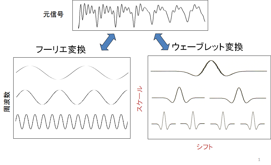
図1.ウェーブレット変換の模式図
出所:https://www.slideshare.net/ryosuketachibana12/ss-42388444
各シフト(時刻),各スケール(周波数)におけるウェーブレットの強さをマッピングしたものをスカログラムと呼びます.図2はy=sin(πx/16)のウェーブレット変換結果から作成したスカログラムです.このようにウェーブレット変換を用いることで任意の波形を画像化することが出来ます.
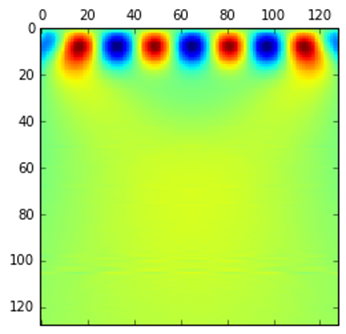
図2.スカログラムの例, y=sin(πx/16)
ウェーブレット変換には連続ウェーブレット変換(CWT)と離散ウェーブレット変換(DWT)がありますが,今回は連続ウェーブレット変換を使用しました.またウェーブレットには色々な形がありますが,とりあえずガウス関数を使用しています.
為替データからスカログラムを作成する
USD/JPYの5分足の終値からスカログラムを作成しました.数年間という膨大なデータから24時間のデータを抽出し,1枚のスカログラムを作成する,という手順を何回も繰り返しました.1枚のスカログラムとその最終時刻の30分後の値動き(上がるor下がる)が1つのデータセットになります.
ここで,1つ問題がありました.スカログラムの境界(端部)にゆがみが生じてしまうことです.これは,境界を越えるとデータが無くなってしまうために起こります.
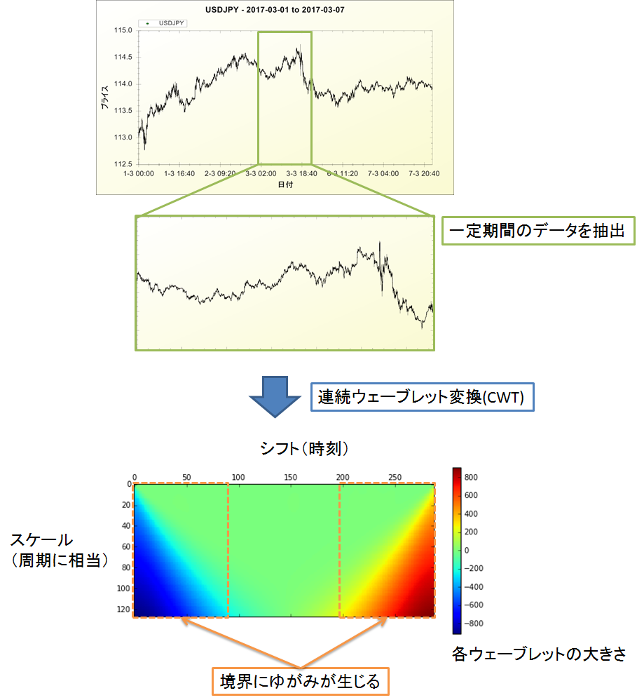
図3.スカログラムの境界に生じるゆがみ
そこでゆがみを除去する為に,生のデータの両端に左右反転したデータを加えました.ウェーブレット変換後に,生のデータに対応する中央部分のみを抽出しました.ゆがみの除去には一般的にこの方法が使われますが,架空のデータを追記していることになりますので,賛否両論ありそうですね.
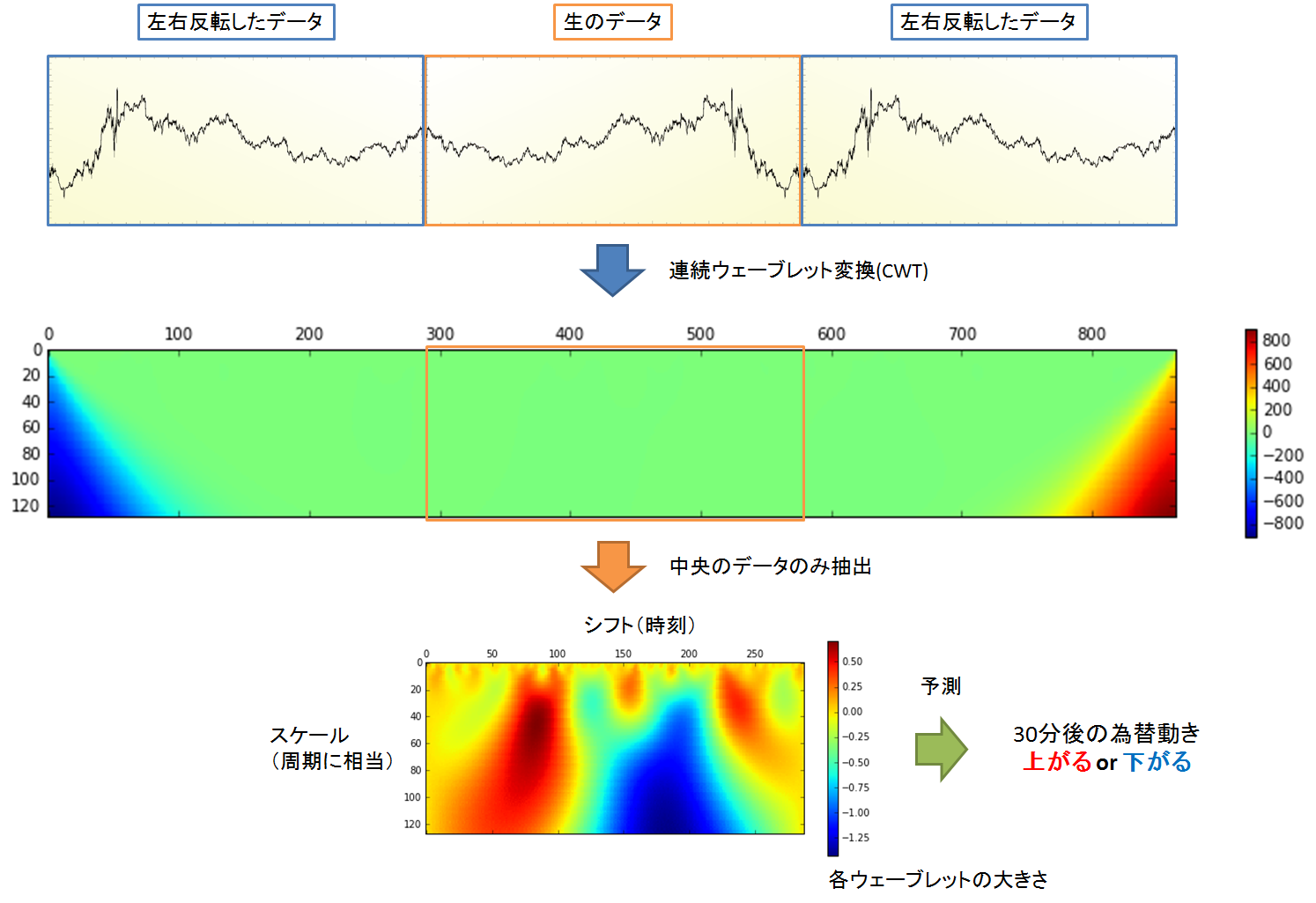
図4.境界に生じるゆがみの除去方法
CNNの構造と学習フロー
学習フローを少し工夫しました.前回までは過去10年間のデータを学習させて,直近の3か月間のデータで精度検証を行いました.今回は過去10年間のデータを学習させた後,過去5年間のデータを学習し,その後は,2年間,1年間と学習データの期間を短くしています.このようにした理由は,未来を予測するためには直近の値動きを重視するべきだと考えた為です.また,テストデータの期間も5か月間に増やしました.テストデータは学習には使用しません.つまり,AIにとって未知のデータとなります.
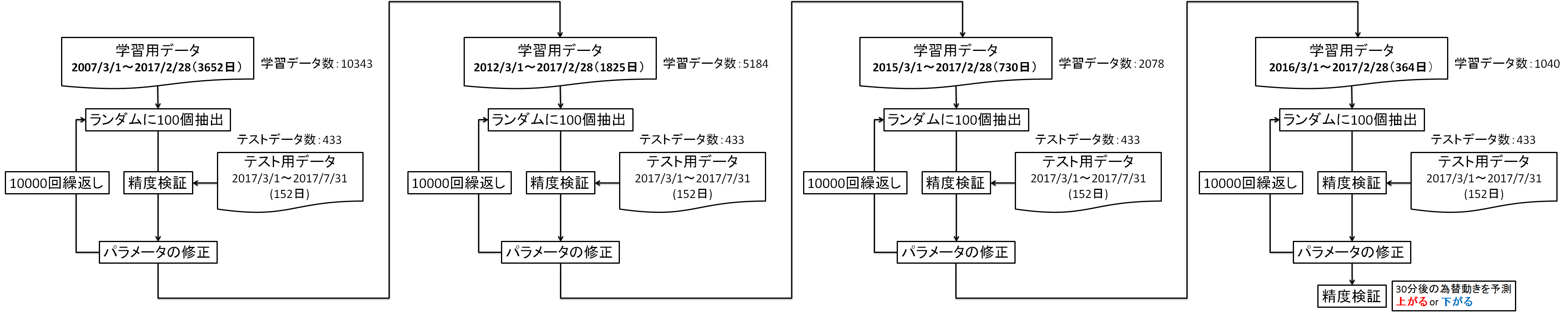
図5.学習フロー
今回使用したCNNの構造を図6に示します.
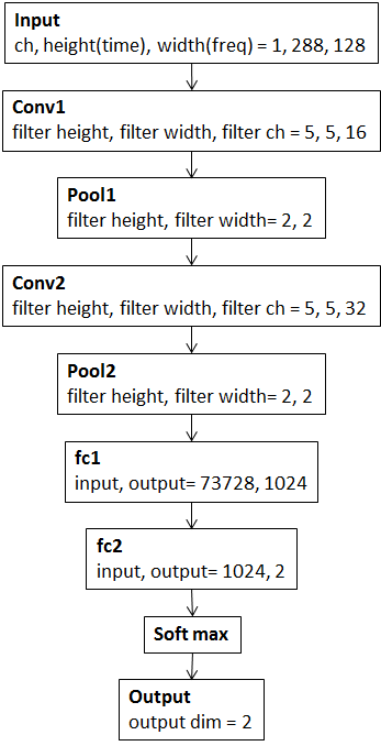
図6.今回使用したCNNの構造
計算結果
という訳で,上手く行ったらいいなぁと思いながらやってみたのですが,結果は図7の通りです.今回もテストデータに対する正解率は上がりませんでした.ちなみに学習データに対する正解率が,Iterations=20000,30000で落ちていますが,これは学習データの期間を切り替えたタイミングと一致しています.
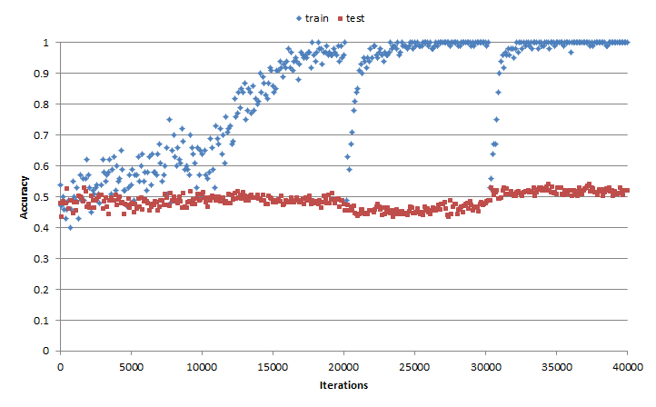
図7.計算結果
おわりに
1枚のスカログラムに含まれる時間情報が一定になっていることが,上手く行かない原因の1つかなぁと思います.今回はどのスカログラムも24時間の波形データから作成しています.実際にトレードしている人たちは,評価する波形の期間を必要に応じて変化させてますよね.
最近「ゲーム理論」に興味が湧いてきて,そっちを勉強中なので為替分析はしばらくお休みしようと思います.
Yu-Nie
Appendix
分析に使用したデータは以下からダウンロードできます.
学習データ
USDJPY_20070301_20170228_5min.csv
USDJPY_20120301_20170228_5min.csv
USDJPY_20150301_20170228_5min.csv
USDJPY_20160301_20170228_5min.csv
テストデータ
USDJPY_20170301_20170731_5min.csv
以下は分析に使用したコードです.
# 20170821
# y.izumi

import tensorflow as tf
import numpy as np
import scalogram2 as sca
import time

"""パラメータの初期化と畳み込み演算,pooling演算を行う関数"""
# =============================================================================================================================================
# 重みの初期化関数
def weight_variable(shape, stddev=1e-4): # default stddev = 1e-4
    initial = tf.truncated_normal(shape, stddev=stddev)
    return tf.Variable(initial)
# バイアスの初期化関数
def bias_variable(shape):
    initial = tf.constant(0.0, shape=shape)
    return tf.Variable(initial)
# 畳み込み演算
def conv2d(x, W):
    return tf.nn.conv2d(x, W, strides=[1, 1, 1, 1], padding="SAME")
# pooling
def max_pool_2x2(x):
    return tf.nn.max_pool(x, ksize=[1, 2, 2, 1], strides=[1, 2, 2, 1], padding="SAME")
# =============================================================================================================================================

"""学習を行う関数"""
# =============================================================================================================================================
def train(x_train, t_train, x_test, t_test, iters, acc_list, num_data_each_conf, acc_each_conf, total_cal_time, train_step, train_batch_size, test_batch_size):
    """
    x_train  : 学習データ
    t_train  : 学習ラベル, one-hot
    x_test   : テストデータ
    t_test   : テストラベル, one-hot
    iters    : 学習回数
    acc_list : 正解率の途中経過を保存するリスト
    num_data_each_conf : 各確信度のデータ数の途中経過を保存するリスト
    acc_each_conf      : 各確信度の正解率の途中経過を保存するリスト
    total_cal_time     : 計算時間の合計
    train_step         : 学習を行うクラス
    train_batch_size   : 学習データのバッチサイズ
    test_batch_size    : テストデータのバッチサイズ
    """
    train_size = x_train.shape[0] # 学習データ数
    test_size = x_test.shape[0]   # テストデータ数
    start_time = time.time()

    iters = iters + 1
    for step in range(iters):
        batch_mask = np.random.choice(train_size, train_batch_size)
        tr_batch_xs = x_train[batch_mask]
        tr_batch_ys = t_train[batch_mask]

        # 学習途中の精度確認
        if step%100 == 0:

            cal_time = time.time() - start_time # 計算時間のカウント
            total_cal_time += cal_time

            # train
            train_accuracy = accuracy.eval(feed_dict={x: tr_batch_xs, y_: tr_batch_ys, keep_prob: 1.0})
            train_loss = cross_entropy.eval(feed_dict={x: tr_batch_xs, y_: tr_batch_ys, keep_prob: 1.0})

            # test
            # use all data
            test_accuracy = accuracy.eval(feed_dict={x: x_test, y_: t_test, keep_prob: 1.0})
            test_loss = cross_entropy.eval(feed_dict={x: x_test, y_: t_test, keep_prob: 1.0})

            # use test batch
            # batch_mask = np.random.choice(test_size, test_batch_size)
            # te_batch_xs = x_test[batch_mask]
            # te_batch_ys = t_test[batch_mask]
            # test_accuracy = accuracy.eval(feed_dict={x: te_batch_xs, y_: te_batch_ys, keep_prob: 1.0})
            # test_loss = cross_entropy.eval(feed_dict={x: te_batch_xs, y_: te_batch_ys, keep_prob: 1.0})

            print("calculation time %d sec, step %d, training accuracy %g, training loss %g, test accuracy %g, test loss %g"%(cal_time, step, train_accuracy, train_loss, test_accuracy, test_loss))
            acc_list.append([step, train_accuracy, test_accuracy, train_loss, test_loss])

            AI_prediction = y_conv.eval(feed_dict={x: x_test, y_: t_test, keep_prob: 1.0}) # AIの予測結果
            # print("AI_prediction.shape " + str(AI_prediction.shape)) # for debag
            # print("AI_prediction.type" + str(type(AI_prediction)))

            AI_correct_prediction = correct_prediction.eval(feed_dict={x: x_test, y_: t_test, keep_prob: 1.0}) # 正解:TRUE, 不正解:FALSE
            # print("AI_prediction.shape " + str(AI_prediction.shape)) # for debag
            # print("AI_prediction.type" + str(type(AI_prediction)))
            AI_correct_prediction_int = AI_correct_prediction.astype(np.int) # 正解:1, 不正解:0

            # 各確信度のデータ数と正解率を計算する
            # 50%以上,60%以下の確信度 (or 40%以上,50%以下の確信度)
            a = AI_prediction[:,0] >= 0.5
            b = AI_prediction[:,0] <= 0.6
            # print("a " + str(a)) # for debag
            # print("a.shape " + str(a.shape))
            cnf_50to60 = np.logical_and(a, b)
            # print("cnf_50to60 " + str(cnf_50to60)) # for debag
            # print("cnf_50to60.shape " + str(cnf_50to60.shape))

            a = AI_prediction[:,0] >= 0.4
            b = AI_prediction[:,0] < 0.5
            cnf_40to50 = np.logical_and(a, b)

            cnf_50to60 = np.logical_or(cnf_50to60, cnf_40to50)
            cnf_50to60_int = cnf_50to60.astype(np.int)
            # print("cnf_50to60_int " + str(cnf_50to60)) # for debag
            # print("cnf_50to60.shape " + str(cnf_50to60.shape))

            correct_prediction_50to60 = np.logical_and(cnf_50to60, AI_correct_prediction)
            correct_prediction_50to60_int = correct_prediction_50to60.astype(np.int)

            sum_50to60 = np.sum(cnf_50to60_int)                             # 確信度が50%から60%のデータ数
            acc_50to60 = np.sum(correct_prediction_50to60_int) / sum_50to60 # 確信度が50%から60%の正解率

            # 60%より大きい,70%以下の確信度 (or 30%以上,40%より小さいの確信度)
            a = AI_prediction[:,0] > 0.6
            b = AI_prediction[:,0] <= 0.7
            cnf_60to70 = np.logical_and(a, b)

            a = AI_prediction[:,0] >= 0.3
            b = AI_prediction[:,0] < 0.4
            cnf_30to40 = np.logical_and(a, b)

            cnf_60to70 = np.logical_or(cnf_60to70, cnf_30to40)
            cnf_60to70_int = cnf_60to70.astype(np.int)

            correct_prediction_60to70 = np.logical_and(cnf_60to70, AI_correct_prediction)
            correct_prediction_60to70_int = correct_prediction_60to70.astype(np.int)

            sum_60to70 = np.sum(cnf_60to70_int)
            acc_60to70 = np.sum(correct_prediction_60to70_int) / sum_60to70

            # 70%より大きい,80%以下の確信度 (or 20%以上,30%より小さいの確信度)
            a = AI_prediction[:,0] > 0.7
            b = AI_prediction[:,0] <= 0.8
            cnf_70to80 = np.logical_and(a, b)

            a = AI_prediction[:,0] >= 0.2
            b = AI_prediction[:,0] < 0.3
            cnf_20to30 = np.logical_and(a, b)

            cnf_70to80 = np.logical_or(cnf_70to80, cnf_20to30)
            cnf_70to80_int = cnf_70to80.astype(np.int)

            correct_prediction_70to80 = np.logical_and(cnf_70to80, AI_correct_prediction)
            correct_prediction_70to80_int = correct_prediction_70to80.astype(np.int)

            sum_70to80 = np.sum(cnf_70to80_int)
            acc_70to80 = np.sum(correct_prediction_70to80_int) / sum_70to80

            # 80%より大きい,90%以下の確信度 (or 10%以上,20%より小さいの確信度)
            a = AI_prediction[:,0] > 0.8
            b = AI_prediction[:,0] <= 0.9
            cnf_80to90 = np.logical_and(a, b)

            a = AI_prediction[:,0] >= 0.1
            b = AI_prediction[:,0] < 0.2
            cnf_10to20 = np.logical_and(a, b)

            cnf_80to90 = np.logical_or(cnf_80to90, cnf_10to20)
            cnf_80to90_int = cnf_80to90.astype(np.int)

            correct_prediction_80to90 = np.logical_and(cnf_80to90, AI_correct_prediction)
            correct_prediction_80to90_int = correct_prediction_80to90.astype(np.int)

            sum_80to90 = np.sum(cnf_80to90_int)
            acc_80to90 = np.sum(correct_prediction_80to90_int) / sum_80to90

            # 90%より大きい,100%以下の確信度 (or 0%以上,10%より小さいの確信度)
            a = AI_prediction[:,0] > 0.9
            b = AI_prediction[:,0] <= 1.0
            cnf_90to100 = np.logical_and(a, b)

            a = AI_prediction[:,0] >= 0
            b = AI_prediction[:,0] < 0.1
            cnf_0to10 = np.logical_and(a, b)

            cnf_90to100 = np.logical_or(cnf_90to100, cnf_0to10)
            cnf_90to100_int = cnf_90to100.astype(np.int)

            correct_prediction_90to100 = np.logical_and(cnf_90to100, AI_correct_prediction)
            correct_prediction_90to100_int = correct_prediction_90to100.astype(np.int)

            sum_90to100 = np.sum(cnf_90to100_int)
            acc_90to100 = np.sum(correct_prediction_90to100_int) / sum_90to100

            print("Number of data of each confidence 50to60:%g, 60to70:%g, 70to80:%g, 80to90:%g, 90to100:%g "%(sum_50to60, sum_60to70, sum_70to80, sum_80to90, sum_90to100))
            print("Accuracy rate of each confidence  50to60:%g, 60to70:%g, 70to80:%g, 80to90:%g, 90to100:%g "%(acc_50to60, acc_60to70, acc_70to80, acc_80to90, acc_90to100))
            print("")

            num_data_each_conf.append([step, sum_50to60, sum_60to70, sum_70to80, sum_80to90, sum_90to100])
            acc_each_conf.append([step, acc_50to60, acc_60to70, acc_70to80, acc_80to90, acc_90to100])

            # tensorboard用ファイルの書き出し
            result = sess.run(merged, feed_dict={x:tr_batch_xs, y_: tr_batch_ys, keep_prob: 1.0})
            writer.add_summary(result, step)

            start_time = time.time()

        # 学習の実行
        train_step.run(feed_dict={x: tr_batch_xs, y_: tr_batch_ys, keep_prob: 0.5})

    return acc_list, num_data_each_conf, acc_each_conf, total_cal_time
# ==============================================================================================================================================

"""スカログラムとラベルを作成する関数"""
# ==============================================================================================================================================
def make_scalogram(train_file_name, test_file_name, scales, wavelet, height, width, predict_time_inc, ch_flag, save_flag, over_lap_inc):
    """
    train_file_name : 学習データのファイル名
    test_file_name  : テストデータのファイル名
    scales  : 使用するスケールをnumpy配列で指定する, スケールは分析に使用するウェーブレットの周波数に相当する, scalesが大きいと低周波, 小さいと高周波になる
    wavelet : ウェーブレットの名前, 以下のいづれかを使用する
              'gaus1', 'gaus2', 'gaus3', 'gaus4', 'gaus5', 'gaus6', 'gaus7', 'gaus8', 'mexh', 'morl'
    height  : 画像の高さ, num of time lines
    width   : 画像の幅,  num of freq lines
    predict_time_inc : 値動きを予測する時刻の増分
    ch_flag      : 使用するチャンネル数, ch_flag=1:close, ch_flag=5:start, high, low, close, volume
    save_flag    : save_flag=1 : CWT係数をcsvファイルとして保存する, save_flag=0 : CWT係数をcsvファイルとして保存しない
    over_lap_inc : CWT開始時刻の増分
    """
    # スカログラムとラベルの作成
    # train
    x_train, t_train, freq_train = sca.merge_scalogram(train_file_name, scales, wavelet, height, width, predict_time_inc, ch_flag, save_flag, over_lap_inc)
    # x_train, t_train, freq_train = sca.merge_scalogram(test_file_name, scales, wavelet, height, width, predict_time_inc, ch_flag, save_flag, over_lap_inc) # for debag
    # test
    x_test, t_test, freq_test = sca.merge_scalogram(test_file_name, scales, wavelet, height, width, predict_time_inc, ch_flag, save_flag, over_lap_inc)
    print("x_train shape " + str(x_train.shape))
    print("t_train shape " + str(t_train.shape))
    print("x_test shape " + str(x_test.shape))
    print("t_test shape " + str(t_test.shape))
    print("frequency " + str(freq_test))

    # tensorflow用に次元を入れ替える
    x_train = x_train.transpose(0, 2, 3, 1) # (num_data, ch, height(time_lines), width(freq_lines)) ⇒ (num_data, height(time_lines), width(freq_lines), ch)
    x_test = x_test.transpose(0, 2, 3, 1)

    train_size = x_train.shape[0]   # 学習データ数
    test_size = x_test.shape[0]     # テストデータ数

    # labes to one-hot
    t_train_onehot = np.zeros((train_size, 2))
    t_test_onehot = np.zeros((test_size, 2))
    t_train_onehot[np.arange(train_size), t_train] = 1
    t_test_onehot[np.arange(test_size), t_test] = 1
    t_train = t_train_onehot
    t_test = t_test_onehot

    # print("t train shape onehot" + str(t_train.shape)) # for debag
    # print("t test shape onehot" + str(t_test.shape))

    return x_train, t_train, x_test, t_test
# ==============================================================================================================================================

"""スカログラムの作成条件"""
# =============================================================================================================================================
predict_time_inc = 6                      # 値動きを予測する時刻の増分
height = 288                              # 画像の高さ, num of time lines
width = 128                               # 画像の幅,  num of freq lines
ch_flag = 1                               # 使用するチャンネル数, ch_flag=1:close, ch_flag=5:start, high, low, close, volume
input_dim = (ch_flag, height, width)      # channel = (1, 5), height(time_lines), width(freq_lines)
save_flag = 0                             # save_flag=1 : CWT係数をcsvファイルとして保存する, save_flag=0 : CWT係数をcsvファイルとして保存しない
scales = np.linspace(0.2,80,width)        # 使用するスケールをnumpy配列で指定する, スケールは分析に使用するウェーブレットの周波数に相当する, scalesが大きいと低周波, 小さいと高周波になる
# scales = np.arange(1,129)
wavelet = "gaus1"                         # ウェーブレットの名前, 'gaus1', 'gaus2', 'gaus3', 'gaus4', 'gaus5', 'gaus6', 'gaus7', 'gaus8', 'mexh', 'morl'
over_lap_inc = 72                         # CWT開始時刻の増分
# ==============================================================================================================================================

"""CNNの構築"""
# ==============================================================================================================================================
x  = tf.placeholder(tf.float32, [None, input_dim[1], input_dim[2], input_dim[0]]) # (num_data, height(time), width(freq_lines), ch)
y_ = tf.placeholder(tf.float32, [None, 2]) # (num_data, num_label)
print("input shape ", str(x.get_shape()))

with tf.variable_scope("conv1") as scope:
    W_conv1 = weight_variable([5, 5, input_dim[0], 16])
    b_conv1 = bias_variable([16])
    h_conv1 = tf.nn.relu(conv2d(x, W_conv1) + b_conv1)
    h_pool1 = max_pool_2x2(h_conv1)
    print("conv1 shape ", str(h_pool1.get_shape()))

with tf.variable_scope("conv2") as scope:
    W_conv2 = weight_variable([5, 5, 16, 32])
    b_conv2 = bias_variable([32])
    h_conv2 = tf.nn.relu(conv2d(h_pool1, W_conv2) + b_conv2)
    h_pool2 = max_pool_2x2(h_conv2)
    print("conv2 shape ", str(h_pool2.get_shape()))
    h_pool2_height = int(h_pool2.get_shape()[1])
    h_pool2_width = int(h_pool2.get_shape()[2])

with tf.variable_scope("fc1") as scope:
    W_fc1 = weight_variable([h_pool2_height*h_pool2_width*32, 1024])
    b_fc1 = bias_variable([1024])
    h_pool2_flat = tf.reshape(h_pool2, [-1, h_pool2_height*h_pool2_width*32])
    h_fc1 = tf.nn.relu(tf.matmul(h_pool2_flat, W_fc1) + b_fc1)
    print("fc1 shape ", str(h_fc1.get_shape()))
    keep_prob = tf.placeholder(tf.float32)
    h_fc1_drop = tf.nn.dropout(h_fc1, keep_prob)

with tf.variable_scope("fc2") as scope:
    W_fc2 = weight_variable([1024, 2])
    b_fc2 = bias_variable([2])
    y_conv = tf.nn.softmax(tf.matmul(h_fc1_drop, W_fc2) + b_fc2)
    print("output shape ", str(y_conv.get_shape()))

# パラメータをtensorboardで可視化する
W_conv1 = tf.summary.histogram("W_conv1", W_conv1)
b_conv1 = tf.summary.histogram("b_conv1", b_conv1)
W_conv2 = tf.summary.histogram("W_conv2", W_conv2)
b_conv2 = tf.summary.histogram("b_conv2", b_conv2)
W_fc1 = tf.summary.histogram("W_fc1", W_fc1)
b_fc1 = tf.summary.histogram("b_fc1", b_fc1)
W_fc2 = tf.summary.histogram("W_fc2", W_fc2)
b_fc2 = tf.summary.histogram("b_fc2", b_fc2)
# ==============================================================================================================================================

"""誤差関数の指定"""
# ==============================================================================================================================================
# cross_entropy = -tf.reduce_sum(y_ * tf.log(y_conv))
cross_entropy = tf.reduce_sum(tf.nn.softmax_cross_entropy_with_logits(labels = y_, logits = y_conv))
loss_summary = tf.summary.scalar("loss", cross_entropy) # for tensorboard
# ==============================================================================================================================================

"""optimizerの指定"""
# ==============================================================================================================================================
optimizer = tf.train.AdamOptimizer(1e-4)
train_step = optimizer.minimize(cross_entropy)

# 勾配をtensorboardで可視化する
grads = optimizer.compute_gradients(cross_entropy)
dW_conv1 = tf.summary.histogram("dW_conv1", grads[0]) # for tensorboard
db_conv1 = tf.summary.histogram("db_conv1", grads[1])
dW_conv2 = tf.summary.histogram("dW_conv2", grads[2])
db_conv2 = tf.summary.histogram("db_conv2", grads[3])
dW_fc1 = tf.summary.histogram("dW_fc1", grads[4])
db_fc1 = tf.summary.histogram("db_fc1", grads[5])
dW_fc2 = tf.summary.histogram("dW_fc2", grads[6])
db_fc2 = tf.summary.histogram("db_fc2", grads[7])

# for i in range(8): # for debag
#     print(grads[i])
# ==============================================================================================================================================

"""精度検証用パラメータ"""
# ==============================================================================================================================================
correct_prediction = tf.equal(tf.argmax(y_conv,1), tf.argmax(y_,1))
accuracy = tf.reduce_mean(tf.cast(correct_prediction, tf.float32))
accuracy_summary = tf.summary.scalar("accuracy", accuracy) # for tensorboard
# ==============================================================================================================================================

"""学習の実行"""
# ==============================================================================================================================================
acc_list = []            # 正解率と誤差の途中経過を保存するリスト
num_data_each_conf = []  # 各確信度のデータ数の途中経過を保存するリスト
acc_each_conf = []       # 各確信度の正解率の途中経過を保存するリスト
start_time = time.time() # 計算時間のカウント
total_cal_time = 0
iters = 10000            # 各学習データに対する学習回数
train_batch_size = 100   # 学習バッチサイズ
test_batch_size = 100    # テストバッチサイズ

with tf.Session() as sess:
    saver = tf.train.Saver()
    sess.run(tf.global_variables_initializer())

    # tensorboard用ファイルの書き出し
    merged = tf.summary.merge_all()
    writer = tf.summary.FileWriter(r"temp_result", sess.graph)

    print("learning term = 10year")
    train_file_name = "USDJPY_20070301_20170228_5min.csv" # 為替データのファイル名, train
    # train_file_name = "USDJPY_20170301_20170731_5min.csv" # for debag
    test_file_name = "USDJPY_20170301_20170731_5min.csv"  # 為替データのファイル名, test
    # スカログラムの作成
    x_train, t_train, x_test, t_test = make_scalogram(train_file_name, test_file_name, scales, wavelet, height, width, predict_time_inc, ch_flag, save_flag, over_lap_inc)
    # 学習の実行
    acc_list, num_data_each_conf, acc_each_conf, total_cal_time = train(x_train, t_train, x_test, t_test, iters, acc_list, num_data_each_conf, acc_each_conf, total_cal_time, train_step, train_batch_size, test_batch_size)

    print("learning term = 5year")
    train_file_name = "USDJPY_20120301_20170228_5min.csv" # 為替データのファイル名, train
    # train_file_name = "USDJPY_20170301_20170731_5min.csv" # for debag
    test_file_name = "USDJPY_20170301_20170731_5min.csv"  # 為替データのファイル名, test
    # スカログラムの作成
    x_train, t_train, x_test, t_test = make_scalogram(train_file_name, test_file_name, scales, wavelet, height, width, predict_time_inc, ch_flag, save_flag, over_lap_inc)
    # 学習の実行
    acc_list, num_data_each_conf, acc_each_conf, total_cal_time = train(x_train, t_train, x_test, t_test, iters, acc_list, num_data_each_conf, acc_each_conf, total_cal_time, train_step, train_batch_size, test_batch_size)

    print("learning term = 2year")
    train_file_name = "USDJPY_20150301_20170228_5min.csv" # 為替データのファイル名, train
    # train_file_name = "USDJPY_20170301_20170731_5min.csv" # for debag
    test_file_name = "USDJPY_20170301_20170731_5min.csv"  # 為替データのファイル名, test
    # スカログラムの作成
    x_train, t_train, x_test, t_test = make_scalogram(train_file_name, test_file_name, scales, wavelet, height, width, predict_time_inc, ch_flag, save_flag, over_lap_inc)
    # 学習の実行
    acc_list, num_data_each_conf, acc_each_conf, total_cal_time = train(x_train, t_train, x_test, t_test, iters, acc_list, num_data_each_conf, acc_each_conf, total_cal_time, train_step, train_batch_size, test_batch_size)

    print("learning term = 1year")
    train_file_name = "USDJPY_20160301_20170228_5min.csv" # 為替データのファイル名, train
    # train_file_name = "USDJPY_20170301_20170731_5min.csv" # for debag
    test_file_name = "USDJPY_20170301_20170731_5min.csv"  # 為替データのファイル名, test
    # スカログラムの作成
    x_train, t_train, x_test, t_test = make_scalogram(train_file_name, test_file_name, scales, wavelet, height, width, predict_time_inc, ch_flag, save_flag, over_lap_inc)
    # 学習の実行
    acc_list, num_data_each_conf, acc_each_conf, total_cal_time = train(x_train, t_train, x_test, t_test, iters, acc_list, num_data_each_conf, acc_each_conf, total_cal_time, train_step, train_batch_size, test_batch_size)

    # テストデータに対する最終正解率
    # use all data
    print("test accuracy %g"%accuracy.eval(feed_dict={x: x_test, y_: t_test, keep_prob: 1.0}))

    # use test batch
    # batch_mask = np.random.choice(test_size, test_batch_size)
    # te_batch_xs = x_test[batch_mask]
    # te_batch_ys = t_test[batch_mask]
    # test_accuracy = accuracy.eval(feed_dict={x: te_batch_xs, y_: te_batch_ys, keep_prob: 1.0})

    print("total calculation time %g sec"%total_cal_time)

    np.savetxt(r"temp_result\acc_list.csv", acc_list, delimiter = ",")                                 # 正解率と誤差の途中経過の書き出し
    np.savetxt(r"temp_result\number_of_data_each_confidence.csv", num_data_each_conf, delimiter = ",") # 各確信度のデータ数の途中経過の書き出し
    np.savetxt(r"temp_result\accuracy_rate_of_each_confidence.csv", acc_each_conf, delimiter = ",")    # 各確信度の正解率の途中経過の書き出し
    saver.save(sess, r"temp_result\spectrogram_model.ckpt")                                            # 最終パラメータの書き出し
# ==============================================================================================================================================
# -*- coding: utf-8 -*-
"""
Created on Tue Jul 25 11:24:50 2017

@author: izumiy
"""

import pywt
import numpy as np
import matplotlib.pyplot as plt

def create_scalogram_1(time_series, scales, wavelet, predict_time_inc, save_flag, ch_flag, height, width):
    """
    連続ウェーブレット変換を実行する関数
    終値を使用
    time_series      : 為替データ, 終値
    scales           : 使用するスケールをnumpy配列で指定する, スケールは分析に使用するウェーブレットの周波数に相当する, scalesが大きいと低周波, 小さいと高周波になる
    wavelet          : ウェーブレットの名前, 以下のいづれかを使用する
     'gaus1', 'gaus2', 'gaus3', 'gaus4', 'gaus5', 'gaus6', 'gaus7', 'gaus8', 'mexh', 'morl'
    predict_time_inc : 値動きを予測する時刻の増分
    save_flag        : save_flag=1 : CWT係数をcsvファイルとして保存する, save_flag=0 : CWT係数をcsvファイルとして保存しない
    ch_flag          : 使用するチャンネル数, ch_flag=1 : close
    height           : 画像の高さ num of time lines
    width            : 画像の幅  num of freq lines
    """

    """為替時系列データの読込み"""
    num_series_data = time_series.shape[0] # データ数の取得
    print("number of the series data : " + str(num_series_data))
    close = time_series

    """連続ウェーブレット変換の実行"""
    # https://pywavelets.readthedocs.io/en/latest/ref/cwt.html
    print("carry out cwt...")
    time_start = 0
    time_end = time_start + height
    scalogram = np.empty((0, ch_flag, height, width))

    # hammingWindow = np.hamming(height)    # ハミング窓
    # hanningWindow = np.hanning(height)    # ハニング窓
    # blackmanWindow = np.blackman(height)  # ブラックマン窓
    # bartlettWindow = np.bartlett(height)  # バートレット窓

    while(time_end <= num_series_data - predict_time_inc):
        # print("time start " + str(time_start)) for debag
        temp_close = close[time_start:time_end]

        # 窓関数有り
        # temp_close = temp_close * hammingWindow

        # ミラー, データの前後に反転したデータを追加する
        mirror_temp_close = temp_close[::-1]
        x = np.append(mirror_temp_close, temp_close)
        temp_close = np.append(x, mirror_temp_close)

        temp_cwt_close, freq_close = pywt.cwt(temp_close, scales, wavelet)        # 連続ウェーブレット変換の実行
        temp_cwt_close = temp_cwt_close.T                                         # 転置 CWT(freq, time) ⇒ CWT(time, freq)

        # ミラー, 中央のデータのみ抽出する
        temp_cwt_close = temp_cwt_close[height:2*height,:]

        temp_cwt_close = np.reshape(temp_cwt_close, (-1, ch_flag, height, width)) # num_data, ch, height(time), width(freq)
        # print("temp_cwt_close_shape " + str(temp_cwt_close.shape)) # for debag
        scalogram = np.append(scalogram, temp_cwt_close, axis=0)
        # print("cwt_close_shape " + str(cwt_close.shape)) # for debag
        time_start = time_end
        time_end = time_start + height

    """ラベルの作成"""
    print("make label...")

    # 2つの配列を比較する方法
    last_time = num_series_data - predict_time_inc
    corrent_close = close[:last_time]
    predict_close = close[predict_time_inc:]
    label_array = predict_close > corrent_close
    # print(label_array[:30]) # for debag

    """
    # whileを使う方法, 遅い
    label_array = np.array([])
    print(label_array)
    time_start = 0
    time_predict = time_start + predict_time_inc

    while(time_predict < num_series_data):
        if close[time_start] >= close[time_predict]:
            label = 0 # 下がる
        else:
            label = 1 # 上がる

        label_array = np.append(label_array, label)
        time_start = time_start + 1
        time_predict = time_start + predict_time_inc
    # print(label_array[:30]) # for debag
    """

    """label_array(time), timeがheightで割り切れる様にスライスする"""
    raw_num_shift = label_array.shape[0]
    num_shift = int(raw_num_shift / height) * height
    label_array = label_array[0:num_shift]

    """各スカログラムに対応したラベルの抽出, (データ数, ラベル)"""
    col = height - 1
    label_array = np.reshape(label_array, (-1, height))
    label_array = label_array[:, col]

    """ファイル出力"""
    if save_flag == 1:
        print("output the files")
        save_cwt_close = np.reshape(scalogram, (-1, width))
        np.savetxt("scalogram.csv", save_cwt_close, delimiter = ",")
        np.savetxt("label.csv", label_array.T, delimiter = ",")

    print("CWT is done")
    return scalogram, label_array, freq_close

def create_scalogram_5(time_series, scales, wavelet, predict_time_inc, save_flag, ch_flag, height, width):
    """
    連続ウェーブレット変換を実行する関数
    終値を使用
    time_series      : 為替データ, 終値
    scales           : 使用するスケールをnumpy配列で指定する, スケールは分析に使用するウェーブレットの周波数に相当する, scalesが大きいと低周波, 小さいと高周波になる
    wavelet          : ウェーブレットの名前, 以下のいづれかを使用する
     'gaus1', 'gaus2', 'gaus3', 'gaus4', 'gaus5', 'gaus6', 'gaus7', 'gaus8', 'mexh', 'morl'
    predict_time_inc : 値動きを予測する時刻の増分
    save_flag        : save_flag=1 : CWT係数をcsvファイルとして保存する, save_flag=0 : CWT係数をcsvファイルとして保存しない
    ch_flag          : 使用するチャンネル数, ch_flag=5 : start, high, low, close, volume
    height           : 画像の高さ num of time lines
    width            : 画像の幅  num of freq lines
    """

    """為替時系列データの読込み"""
    num_series_data = time_series.shape[0] # データ数の取得
    print("number of the series data : " + str(num_series_data))
    start = time_series[:,0]
    high = time_series[:,1]
    low = time_series[:,2]
    close = time_series[:,3]
    volume = time_series[:,4]

    """連続ウェーブレット変換の実行"""
    # https://pywavelets.readthedocs.io/en/latest/ref/cwt.html
    print("carry out cwt...")
    time_start = 0
    time_end = time_start + height
    scalogram = np.empty((0, ch_flag, height, width))

    while(time_end <= num_series_data - predict_time_inc):
        # print("time start " + str(time_start)) for debag
        temp_start = start[time_start:time_end]
        temp_high = high[time_start:time_end]
        temp_low = low[time_start:time_end]
        temp_close = close[time_start:time_end]
        temp_volume = volume[time_start:time_end]

        temp_cwt_start, freq_start = pywt.cwt(temp_start, scales, wavelet)        # 連続ウェーブレット変換の実行
        temp_cwt_high, freq_high = pywt.cwt(temp_high, scales, wavelet)
        temp_cwt_low, freq_low = pywt.cwt(temp_low, scales, wavelet)
        temp_cwt_close, freq_close = pywt.cwt(temp_close, scales, wavelet)
        temp_cwt_volume, freq_volume = pywt.cwt(temp_volume, scales, wavelet)

        temp_cwt_start = temp_cwt_start.T                                         # 転置 CWT(freq, time) ⇒ CWT(time, freq)
        temp_cwt_high = temp_cwt_high.T
        temp_cwt_low = temp_cwt_low.T
        temp_cwt_close = temp_cwt_close.T
        temp_cwt_volume = temp_cwt_volume.T

        temp_cwt_start = np.reshape(temp_cwt_start, (-1, 1, height, width)) # num_data, ch, height(time), width(freq)
        temp_cwt_high = np.reshape(temp_cwt_high, (-1, 1, height, width))
        temp_cwt_low = np.reshape(temp_cwt_low, (-1, 1, height, width))
        temp_cwt_close = np.reshape(temp_cwt_close, (-1, 1, height, width))
        temp_cwt_volume = np.reshape(temp_cwt_volume, (-1, 1, height, width))
        # print("temp_cwt_close_shape " + str(temp_cwt_close.shape)) # for debag

        temp_cwt_start = np.append(temp_cwt_start, temp_cwt_high, axis=1)
        temp_cwt_start = np.append(temp_cwt_start, temp_cwt_low, axis=1)
        temp_cwt_start = np.append(temp_cwt_start, temp_cwt_close, axis=1)
        temp_cwt_start = np.append(temp_cwt_start, temp_cwt_volume, axis=1)
        # print("temp_cwt_start_shape " + str(temp_cwt_start.shape)) for debag

        scalogram = np.append(scalogram, temp_cwt_start, axis=0)
        # print("cwt_close_shape " + str(cwt_close.shape)) # for debag
        time_start = time_end
        time_end = time_start + height

    """ラベルの作成"""
    print("make label...")

    # 2つの配列を比較する方法
    last_time = num_series_data - predict_time_inc
    corrent_close = close[:last_time]
    predict_close = close[predict_time_inc:]
    label_array = predict_close > corrent_close
    # print(label_array[:30]) # for debag

    """
    # whileを使う方法, 遅い
    label_array = np.array([])
    print(label_array)
    time_start = 0
    time_predict = time_start + predict_time_inc

    while(time_predict < num_series_data):
        if close[time_start] >= close[time_predict]:
            label = 0 # 下がる
        else:
            label = 1 # 上がる

        label_array = np.append(label_array, label)
        time_start = time_start + 1
        time_predict = time_start + predict_time_inc
    # print(label_array[:30]) # for debag
    """

    """label_array(time), timeがheightで割り切れる様にスライスする"""
    raw_num_shift = label_array.shape[0]
    num_shift = int(raw_num_shift / height) * height
    label_array = label_array[0:num_shift]

    """各スカログラムに対応したラベルの抽出, (データ数, ラベル)"""
    col = height - 1
    label_array = np.reshape(label_array, (-1, height))
    label_array = label_array[:, col]

    """ファイル出力"""
    if save_flag == 1:
        print("output the files")
        save_cwt_close = np.reshape(scalogram, (-1, width))
        np.savetxt("scalogram.csv", save_cwt_close, delimiter = ",")
        np.savetxt("label.csv", label_array.T, delimiter = ",")

    print("CWT is done")
    return scalogram, label_array, freq_close

def CWT_1(time_series, scales, wavelet, predict_time_inc, save_flag):
    """
    連続ウェーブレット変換を実行する関数
    終値を使用
    time_series      : 為替データ, 終値
    scales           : 使用するスケールをnumpy配列で指定する, スケールは分析に使用するウェーブレットの周波数に相当する, scalesが大きいと低周波, 小さいと高周波になる
    wavelet          : ウェーブレットの名前, 以下のいづれかを使用する
     'gaus1', 'gaus2', 'gaus3', 'gaus4', 'gaus5', 'gaus6', 'gaus7', 'gaus8', 'mexh', 'morl'
    predict_time_inc : 値動きを予測する時刻の増分
    save_flag        : save_flag=1 : CWT係数をcsvファイルとして保存する, save_flag=0 : CWT係数をcsvファイルとして保存しない
    """

    """為替時系列データの読込み"""
    num_series_data = time_series.shape[0] # データ数の取得
    print("number of the series data : " + str(num_series_data))
    close = time_series

    """連続ウェーブレット変換の実行"""
    # https://pywavelets.readthedocs.io/en/latest/ref/cwt.html
    print("carry out cwt...")
    cwt_close, freq_close = pywt.cwt(close, scales, wavelet)

    # 転置 CWT(freq, time) ⇒ CWT(time, freq)
    cwt_close = cwt_close.T

    """ラベルの作成"""
    print("make label...")

    # 2つの配列を比較する方法
    last_time = num_series_data - predict_time_inc
    corrent_close = close[:last_time]
    predict_close = close[predict_time_inc:]
    label_array = predict_close > corrent_close
    # print(label_array[:30]) # for debag

    """
    # whileを使う方法
    label_array = np.array([])
    print(label_array)
    time_start = 0
    time_predict = time_start + predict_time_inc

    while(time_predict < num_series_data):
        if close[time_start] >= close[time_predict]:
            label = 0 # 下がる
        else:
            label = 1 # 上がる

        label_array = np.append(label_array, label)
        time_start = time_start + 1
        time_predict = time_start + predict_time_inc
    # print(label_array[:30]) # for debag
    """

    """ファイル出力"""
    if save_flag == 1:
        print("output the files")
        np.savetxt("CWT_close.csv", cwt_close, delimiter = ",")
        np.savetxt("label.csv", label_array.T, delimiter = ",")

    print("CWT is done")
    return [cwt_close], label_array, freq_close

def merge_CWT_1(cwt_list, label_array, height, width):
    """
    終値を使用
    cwt_list    : CWTの結果リスト
    label_array : ラベルを格納したnumpy配列
    height      : 画像の高さ num of time lines
    width       : 画像の幅  num of freq lines
    """
    print("merge CWT")

    cwt_close = cwt_list[0]  # 終値 CWT(time, freq)

    """CWT(time, freq), timeがheightで割り切れる様にスライスする"""
    raw_num_shift = cwt_close.shape[0]
    num_shift = int(raw_num_shift / height) * height
    cwt_close = cwt_close[0:num_shift]
    label_array = label_array[0:num_shift]

    """形状変更, (データ数, チャンネル, 高さ(time), 幅(freq))"""
    cwt_close = np.reshape(cwt_close, (-1, 1, height, width))

    """各スカログラムに対応したラベルの抽出, (データ数, ラベル)"""
    col = height - 1
    label_array = np.reshape(label_array, (-1, height))
    label_array = label_array[:, col]

    return cwt_close, label_array

def CWT_2(time_series, scales, wavelet, predict_time_inc, save_flag):
    """
    連続ウェーブレット変換を実行する関数
    終値,Volumeを使用
    time_series      : 為替データ, 終値, volume
    scales           : 使用するスケールをnumpy配列で指定する, スケールは分析に使用するウェーブレットの周波数に相当する, scalesが大きいと低周波, 小さいと高周波になる
    wavelet          : ウェーブレットの名前, 以下のいづれかを使用する
     'gaus1', 'gaus2', 'gaus3', 'gaus4', 'gaus5', 'gaus6', 'gaus7', 'gaus8', 'mexh', 'morl'
    predict_time_inc : 値動きを予測する時刻の増分
    save_flag        : save_flag=1 : CWT係数をcsvファイルとして保存する, save_flag=0 : CWT係数をcsvファイルとして保存しない
    """

    """為替時系列データの読込み"""
    num_series_data = time_series.shape[0] # データ数の取得
    print("number of the series data : " + str(num_series_data))
    close = time_series[:,0]
    volume = time_series[:,1]

    """連続ウェーブレット変換の実行"""
    # https://pywavelets.readthedocs.io/en/latest/ref/cwt.html
    print("carry out cwt...")
    cwt_close, freq_close = pywt.cwt(close, scales, wavelet)
    cwt_volume, freq_volume = pywt.cwt(volume, scales, wavelet)

    # 転置 CWT(freq, time) ⇒ CWT(time, freq)
    cwt_close = cwt_close.T
    cwt_volume = cwt_volume.T

    """ラベルの作成"""
    print("make label...")

    # 2つの配列を比較する方法
    last_time = num_series_data - predict_time_inc
    corrent_close = close[:last_time]
    predict_close = close[predict_time_inc:]
    label_array = predict_close > corrent_close
    # print(label_array[:30]) # for debag

    """
    # whileを使う方法
    label_array = np.array([])
    print(label_array)
    time_start = 0
    time_predict = time_start + predict_time_inc

    while(time_predict < num_series_data):
        if close[time_start] >= close[time_predict]:
            label = 0 # 下がる
        else:
            label = 1 # 上がる

        label_array = np.append(label_array, label)
        time_start = time_start + 1
        time_predict = time_start + predict_time_inc
    # print(label_array[:30]) # for debag
    """

    """ファイル出力"""
    if save_flag == 1:
        print("output the files")
        np.savetxt("CWT_close.csv", cwt_close, delimiter = ",")
        np.savetxt("CWT_volume.csv", cwt_volume, delimiter = ",")
        np.savetxt("label.csv", label_array.T, delimiter = ",")

    print("CWT is done")
    return [cwt_close, cwt_volume], label_array, freq_close

def merge_CWT_2(cwt_list, label_array, height, width):
    """
    終値,Volumeを使用
    cwt_list    : CWTの結果リスト
    label_array : ラベルを格納したnumpy配列
    height      : 画像の高さ num of time lines
    width       : 画像の幅  num of freq lines
    """
    print("merge CWT")

    cwt_close = cwt_list[0]  # 終値 CWT(time, freq)
    cwt_volume = cwt_list[1] # 出来高

    """CWT(time, freq), timeがheightで割り切れる様にスライスする"""
    raw_num_shift = cwt_close.shape[0]
    num_shift = int(raw_num_shift / height) * height
    cwt_close = cwt_close[0:num_shift]
    cwt_volume = cwt_volume[0:num_shift]
    label_array = label_array[0:num_shift]

    """形状変更, (データ数, チャンネル, 高さ(time), 幅(freq))"""
    cwt_close = np.reshape(cwt_close, (-1, 1, height, width))
    cwt_volume = np.reshape(cwt_volume, (-1, 1, height, width))

    """マージする"""
    cwt_close = np.append(cwt_close, cwt_volume, axis=1)

    """各スカログラムに対応したラベルの抽出, (データ数, ラベル)"""
    col = height - 1
    label_array = np.reshape(label_array, (-1, height))
    label_array = label_array[:, col]

    return cwt_close, label_array

def CWT_5(time_series, scales, wavelet, predict_time_inc, save_flag):
    """
    連続ウェーブレット変換を実行する関数
    始値,高値,安値,終値,Volumeを使用
    time_series      : 為替データ, 始値, 高値, 安値, 終値, volume
    scales           : 使用するスケールをnumpy配列で指定する, スケールは分析に使用するウェーブレットの周波数に相当する, scalesが大きいと低周波, 小さいと高周波になる
    wavelet          : ウェーブレットの名前, 以下のいづれかを使用する
     'gaus1', 'gaus2', 'gaus3', 'gaus4', 'gaus5', 'gaus6', 'gaus7', 'gaus8', 'mexh', 'morl'
    predict_time_inc : 値動きを予測する時刻の増分
    save_flag        : save_flag=1 : CWT係数をcsvファイルとして保存する, save_flag=0 : CWT係数をcsvファイルとして保存しない
    """

    """為替時系列データの読込み"""
    num_series_data = time_series.shape[0] # データ数の取得
    print("number of the series data : " + str(num_series_data))
    start = time_series[:,0]
    high = time_series[:,1]
    low = time_series[:,2]
    close = time_series[:,3]
    volume = time_series[:,4]

    """連続ウェーブレット変換の実行"""
    # https://pywavelets.readthedocs.io/en/latest/ref/cwt.html
    print("carry out cwt...")
    cwt_start, freq_start = pywt.cwt(start, scales, wavelet)
    cwt_high, freq_high = pywt.cwt(high, scales, wavelet)
    cwt_low, freq_low = pywt.cwt(low, scales, wavelet)
    cwt_close, freq_close = pywt.cwt(close, scales, wavelet)
    cwt_volume, freq_volume = pywt.cwt(volume, scales, wavelet)

    # 転置 CWT(freq, time) ⇒ CWT(time, freq)
    cwt_start = cwt_start.T
    cwt_high = cwt_high.T
    cwt_low = cwt_low.T
    cwt_close = cwt_close.T
    cwt_volume = cwt_volume.T

    """ラベルの作成"""
    print("make label...")

    # 2つの配列を比較する方法
    last_time = num_series_data - predict_time_inc
    corrent_close = close[:last_time]
    predict_close = close[predict_time_inc:]
    label_array = predict_close > corrent_close
    # print(label_array.dtype) >>> bool

    """
    # whileを使う方法
    label_array = np.array([])
    print(label_array)
    time_start = 0
    time_predict = time_start + predict_time_inc

    while(time_predict < num_series_data):
        if close[time_start] >= close[time_predict]:
            label = 0 # 下がる
        else:
            label = 1 # 上がる

        label_array = np.append(label_array, label)
        time_start = time_start + 1
        time_predict = time_start + predict_time_inc
    # print(label_array[:30]) # for debag
    """

    """ファイル出力"""
    if save_flag == 1:
        print("output the files")
        np.savetxt("CWT_start.csv", cwt_start, delimiter = ",")
        np.savetxt("CWT_high.csv", cwt_high, delimiter = ",")
        np.savetxt("CWT_low.csv", cwt_low, delimiter = ",")
        np.savetxt("CWT_close.csv", cwt_close, delimiter = ",")
        np.savetxt("CWT_volume.csv", cwt_volume, delimiter = ",")
        np.savetxt("label.csv", label_array.T, delimiter = ",")

    print("CWT is done")
    return [cwt_start, cwt_high, cwt_low, cwt_close, cwt_volume], label_array, freq_close

def merge_CWT_5(cwt_list, label_array, height, width):
    """
    cwt_list    : CWTの結果リスト
    label_array : ラベルを格納したnumpy配列
    height      : 画像の高さ num of time lines
    width       : 画像の幅  num of freq lines
    """
    print("merge CWT")

    cwt_start = cwt_list[0]  # 始値
    cwt_high = cwt_list[1]   # 高値
    cwt_low = cwt_list[2]    # 安値
    cwt_close = cwt_list[3]  # 終値 CWT(time, freq)
    cwt_volume = cwt_list[4] # 出来高

    """CWT(time, freq), timeがheightで割り切れる様にスライスする"""
    raw_num_shift = cwt_close.shape[0]
    num_shift = int(raw_num_shift / height) * height
    cwt_start = cwt_start[0:num_shift]
    cwt_high = cwt_high[0:num_shift]
    cwt_low = cwt_low[0:num_shift]
    cwt_close = cwt_close[0:num_shift]
    cwt_volume = cwt_volume[0:num_shift]
    label_array = label_array[0:num_shift]

    """形状変更, (データ数, チャンネル, 高さ(time), 幅(freq))"""
    cwt_start = np.reshape(cwt_start, (-1, 1, height, width))
    cwt_high = np.reshape(cwt_high, (-1, 1, height, width))
    cwt_low = np.reshape(cwt_low, (-1, 1, height, width))
    cwt_close = np.reshape(cwt_close, (-1, 1, height, width))
    cwt_volume = np.reshape(cwt_volume, (-1, 1, height, width))

    """マージする"""
    cwt_start = np.append(cwt_start, cwt_high, axis=1)
    cwt_start = np.append(cwt_start, cwt_low, axis=1)
    cwt_start = np.append(cwt_start, cwt_close, axis=1)
    cwt_start = np.append(cwt_start, cwt_volume, axis=1)

    """各スカログラムに対応したラベルの抽出, (データ数, ラベル)"""
    col = height - 1
    label_array = np.reshape(label_array, (-1, height))
    label_array = label_array[:, col]
    # print(label_array.dtype) >>> bool

    return cwt_start, label_array

def make_scalogram(input_file_name, scales, wavelet, height, width, predict_time_inc, ch_flag, save_flag, over_lap_inc):
    """
    input_file_name  : 為替データのファイル名
    scales           : 使用するスケールをnumpy配列で指定する, スケールは分析に使用するウェーブレットの周波数に相当する, scalesが大きいと低周波, 小さいと高周波になる
    wavelet          : ウェーブレットの名前, 以下のいづれかを使用する
     'gaus1', 'gaus2', 'gaus3', 'gaus4', 'gaus5', 'gaus6', 'gaus7', 'gaus8', 'mexh', 'morl'
    predict_time_inc : 値動きを予測する時刻の増分
    height           : 画像の高さ num of time lines
    width            : 画像の幅  num of freq lines
    ch_flag          : 使用するチャンネル数, ch_flag=1:close, ch_flag=2:close and volume, ch_flag=5:start, high, low, close, volume
    save_flag        : save_flag=1 : CWT係数をcsvファイルとして保存する, save_flag=0 : CWT係数をcsvファイルとして保存しない
    over_lap_inc     : CWT開始時刻の増分
    """

    scalogram = np.empty((0, ch_flag, height, width)) # 全てのスカログラムとラベルを格納する配列
    label = np.array([])
    over_lap_start = 0
    over_lap_end = int((height - 1) / over_lap_inc) * over_lap_inc + 1

    if ch_flag==1:

        print("reading the input file...")
        time_series = np.loadtxt(input_file_name, delimiter = ",", usecols = (5,), skiprows = 1) # 終値をnumpy配列として取得する

        for i in range(over_lap_start, over_lap_end, over_lap_inc):
            print("over_lap_start " + str(i))
            temp_time_series = time_series[i:] # CWTの開始時刻を変化させる
            cwt_list, label_array, freq = CWT_1(temp_time_series, scales, wavelet, predict_time_inc, save_flag) # CWTの実行
            temp_scalogram, temp_label = merge_CWT_1(cwt_list, label_array, height, width)                      # スカログラムの作成

            scalogram = np.append(scalogram, temp_scalogram, axis=0) # 全てのスカログラムとラベルを1つの配列にまとめる
            label = np.append(label, temp_label)

        print("scalogram_shape " + str(scalogram.shape))
        print("label shape " + str(label.shape))
        print("frequency " + str(freq))

    elif ch_flag==2:

        print("reading the input file...")
        time_series = np.loadtxt(input_file_name, delimiter = ",", usecols = (5,6), skiprows = 1) # 終値,volumeをnumpy配列として取得する

        for i in range(over_lap_start, over_lap_end, over_lap_inc):
            print("over_lap_start " + str(i))
            temp_time_series = time_series[i:] # CWTの開始時刻を変化させる
            cwt_list, label_array, freq = CWT_2(temp_time_series, scales, wavelet, predict_time_inc, save_flag) # CWTの実行
            temp_scalogram, temp_label = merge_CWT_2(cwt_list, label_array, height, width)                      # スカログラムの作成

            scalogram = np.append(scalogram, temp_scalogram, axis=0) # 全てのスカログラムとラベルを1つの配列にまとめる
            label = np.append(label, temp_label)

        print("scalogram_shape " + str(scalogram.shape))
        print("label shape " + str(label.shape))
        print("frequency " + str(freq))

    elif ch_flag==5:

        print("reading the input file...")
        time_series = np.loadtxt(input_file_name, delimiter = ",", usecols = (2,3,4,5,6), skiprows = 1) # 始値,高値,安値,終値,volumeをnumpy配列として取得する

        for i in range(over_lap_start, over_lap_end, over_lap_inc):
            print("over_lap_start " + str(i))
            temp_time_series = time_series[i:] # CWTの開始時刻を変化させる
            cwt_list, label_array, freq = CWT_5(temp_time_series, scales, wavelet, predict_time_inc, save_flag) # CWTの実行
            temp_scalogram, temp_label = merge_CWT_5(cwt_list, label_array, height, width)                      # スカログラムの作成

            scalogram = np.append(scalogram, temp_scalogram, axis=0) # 全てのスカログラムとラベルを1つの配列にまとめる
            label = np.append(label, temp_label)
            # print(temp_label.dtype) >>> bool
            # print(label.dtype)      >>> float64

        print("scalogram_shape " + str(scalogram.shape))
        print("label shape " + str(label.shape))
        print("frequency " + str(freq))

    label = label.astype(np.int)
    return scalogram, label

def merge_scalogram(input_file_name, scales, wavelet, height, width, predict_time_inc, ch_flag, save_flag, over_lap_inc):
    """
    input_file_name  : 為替データのファイル名
    scales           : 使用するスケールをnumpy配列で指定する, スケールは分析に使用するウェーブレットの周波数に相当する, scalesが大きいと低周波, 小さいと高周波になる
    wavelet          : ウェーブレットの名前, 以下のいづれかを使用する
     'gaus1', 'gaus2', 'gaus3', 'gaus4', 'gaus5', 'gaus6', 'gaus7', 'gaus8', 'mexh', 'morl'
    predict_time_inc : 値動きを予測する時刻の増分
    height           : 画像の高さ num of time lines
    width            : 画像の幅  num of freq lines
    ch_flag          : 使用するチャンネル数, ch_flag=1:close, ch_flag=2:close and volume, ch_flag=5:start, high, low, close, volume
    save_flag        : save_flag=1 : CWT係数をcsvファイルとして保存する, save_flag=0 : CWT係数をcsvファイルとして保存しない
    over_lap_inc     : CWT開始時刻の増分
    """

    scalogram = np.empty((0, ch_flag, height, width)) # 全てのスカログラムとラベルを格納する配列
    label = np.array([])
    over_lap_start = 0
    over_lap_end = int((height - 1) / over_lap_inc) * over_lap_inc + 1

    if ch_flag==1:

        print("reading the input file...")
        time_series = np.loadtxt(input_file_name, delimiter = ",", usecols = (5,), skiprows = 1) # 終値をnumpy配列として取得する

        for i in range(over_lap_start, over_lap_end, over_lap_inc):
            print("over_lap_start " + str(i))
            temp_time_series = time_series[i:] # CWTの開始時刻を変化させる
            temp_scalogram, temp_label, freq = create_scalogram_1(temp_time_series, scales, wavelet, predict_time_inc, save_flag, ch_flag, height, width)
            scalogram = np.append(scalogram, temp_scalogram, axis=0) # 全てのスカログラムとラベルを1つの配列にまとめる
            label = np.append(label, temp_label)

        # print("scalogram_shape " + str(scalogram.shape))
        # print("label shape " + str(label.shape))
        # print("frequency " + str(freq))

    if ch_flag==5:

        print("reading the input file...")
        time_series = np.loadtxt(input_file_name, delimiter = ",", usecols = (2,3,4,5,6), skiprows = 1) # 終値をnumpy配列として取得する

        for i in range(over_lap_start, over_lap_end, over_lap_inc):
            print("over_lap_start " + str(i))
            temp_time_series = time_series[i:] # CWTの開始時刻を変化させる
            temp_scalogram, temp_label, freq = create_scalogram_5(temp_time_series, scales, wavelet, predict_time_inc, save_flag, ch_flag, height, width)
            scalogram = np.append(scalogram, temp_scalogram, axis=0) # 全てのスカログラムとラベルを1つの配列にまとめる
            label = np.append(label, temp_label)

    label = label.astype(np.int)
    return scalogram, label, freq