はじめに
この手法はまだ良い結果が得られていません.趣味としてアイデアを試している段階ですので,直ぐに使えるツールをお探しの方のお役には立てないと思います.ご了承下さい.m(__)m
さて,前回記事ではスペクトログラムという音分析技術で為替データ(USD/JPY)を画像化し,CNNで学習しました.10枚のスペクトログラムと1分後の終値の値動き(上がるor下がる)を1つのデータセットとし,過去の為替データから学習データ:57864個,テストデータ:1453個を用意しました.
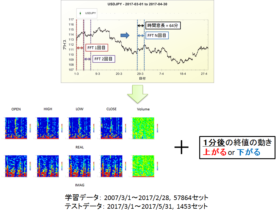
図1.前回使用した学習データの例
前回の結果が図2になります.テストデータに対する予測精度は全然上がりませんでした.
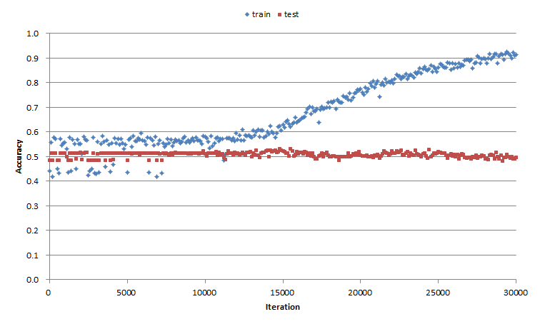
図2.前回の精度検証結果
前回と違うところ
今回も基本的な考え方は同じですが,以下の2点が異なります.
学習データの調整
表1に変更点をまとめました.1番大きな違いはFFTのサンプリング数を増やして,より低い周波数の波に分解したことです.低周波に着目した理由は,前回作成したスペクトログラムを見ると,桁違いに強い応答が出ていたからです.
また,使用するデータを終値のみとしました.低周波まで分解したことで,スペクトログラムのサイズが大きくなり,メモリが足りなくなってしまいました(笑).
表1.学習データの比較
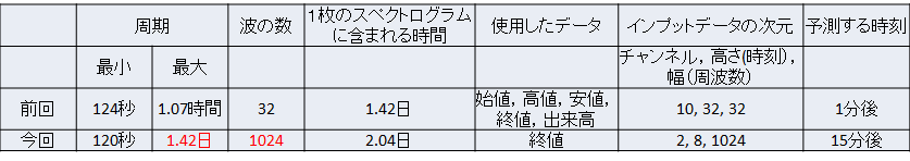
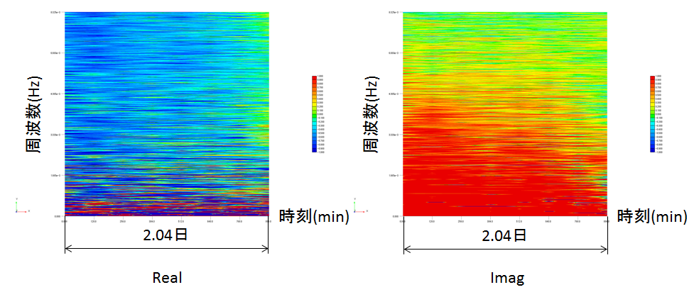
図3.今回使用した学習データの例
Tensor Flowを使用
スペクトログラムのサイズが大きくなったことで,学習に1週間以上掛かる様になりました.ハイパーパラメータの条件出しは本番よりも軽い計算条件で行いますが,それでも時間が掛かり過ぎます.そこで,Tensor FlowのGPU環境に乗り換えました.速いです.1晩で学習が終わる様になりました.
計算フロー
CNNの構造を図4に示します.学習フローは図5になります.
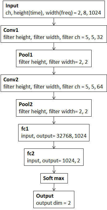
図4.CNNの構造
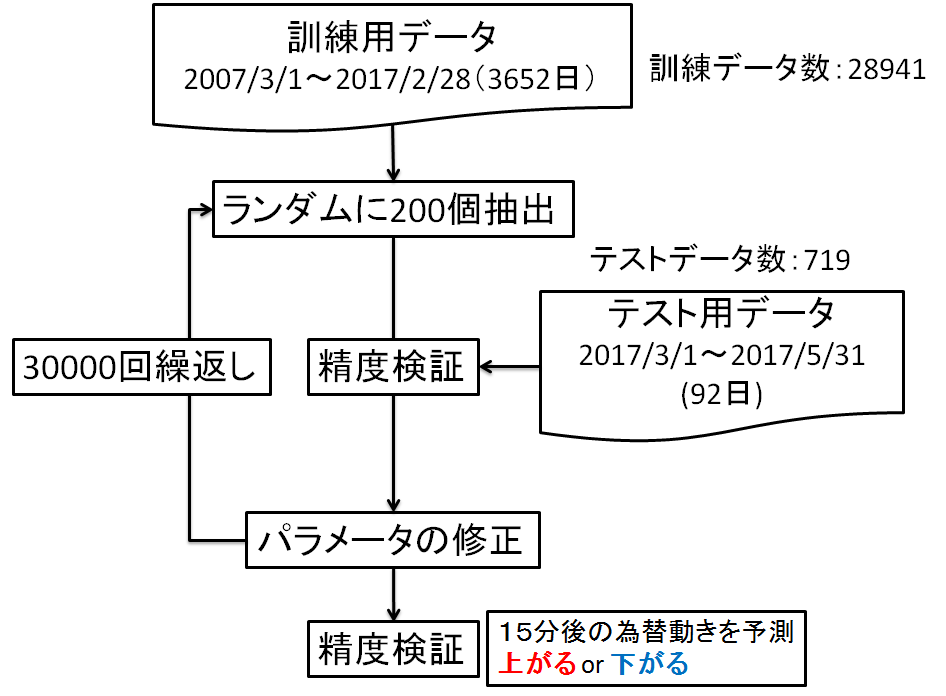
図5.学習フロー
計算結果
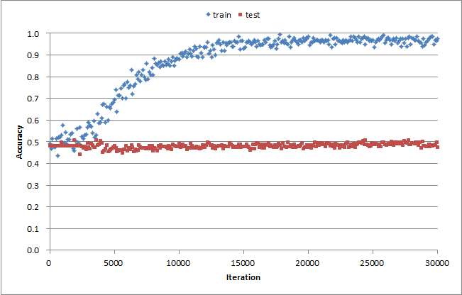
今回もテストデータに対する正解率が上がりませんでした...残念!
所感
他の金融データも学習データに取り入れたい
例えば,USD/JPYを予測するのにUSD/JPYだけでなく,EUR/JPYも考慮してみる,というアプローチは必要かなぁ,と思っています.通貨だけでなく,株式や国債,貴金属の価格なども影響していると思います.全部ぶっこみたいところですが,計算コストがどんどん増大することがネックですね.(^_^;)
そもそも為替データをFFTすることにどんな物理的意味があるの?
この取組では以下の仮定が正しいか検証しているのですが,
「為替データをsin波の重ね合わせで表現した時に,各波の強さと位相,そしてその履歴は将来の為替の値動きと相関がある.」
そもそも為替データをFFTすることにどんな物理的な意味があるのでしょうか?あんまり考えてませんでした(笑).過去の文献に何か情報無いか調べてみます.
Yu-Nie
Appendix
分析対象とした為替データは以下からダウンロードできます.
USDJPY_20070301_20170228_1min.csv
USDJPY_20170301_20170531_1min.csv
以下は分析に使用したコードです.
# 20170719
# y.izumi

import tensorflow as tf
import numpy as np
import spectrogram as spec # FFTとスペクトログラム作成を行うためのモジュール
import time

"""パラメータの初期化と畳み込み演算,pooling演算を行う関数"""
# =============================================================================================================================================
# 重みの初期化関数
def weight_variable(shape, stddev=1e-5): # default stddev = 1e-4
    initial = tf.truncated_normal(shape, stddev=stddev)
    return tf.Variable(initial)
# バイアスの初期化関数
def bias_variable(shape):
    initial = tf.constant(0.0, shape=shape)
    return tf.Variable(initial)
# 畳み込み演算
def conv2d(x, W):
    return tf.nn.conv2d(x, W, strides=[1, 1, 1, 1], padding="SAME")
# pooling
def max_pool_2x2(x):
    return tf.nn.max_pool(x, ksize=[1, 2, 2, 1], strides=[1, 2, 2, 1], padding="SAME")
# =============================================================================================================================================

"""スペクトログラムの作成条件"""
# =============================================================================================================================================
tr_raw_file_name = "USDJPY_20070301_20170228_1min.csv"                     # 生データファイル名 train
tr_spectrogram_file_name = "USDJPY_20070301_20170228_1min_spectrogram.csv" # FFT結果のファイル名 train
te_raw_file_name = "USDJPY_20170301_20170531_1min.csv"                     # 生データファイル名 test
te_spectrogram_file_name = "USDJPY_20170301_20170531_1min_spectrogram.csv" # FFT結果のファイル名 test
FFT_num_sample = 2048                   # 1回のFFTに使用するサンプル数(注意)2の乗数にすること
FFT_over_lap = 16                       # FFT_time_inc = FFT_num_sample / FFT_over_lap, FFT_time_incはFFTの開始時刻の増分
predict_time_inc = 15                   # 15分後の為替が上がるor下がるを予測する
time_lines = 8                          # 1枚のスペクトログラムに含まれるFFTの数
freq_lines = int(FFT_num_sample / 2)    # 1枚のスペクトログラムに踏まれる周波数の数
input_dim = (2, time_lines, freq_lines) # channel(= 2, 4, 6, 8, 10), height(time), width(freq_lines)
ch_flag = input_dim[0]
# 各チャンネルは以下の値からスペクトログラムを作成します
# ch_flag = 2 : (close) x (real, imag)
# ch_flag = 4 : (close, volume) x (real, imag)
# ch_flag = 6 : (high, low, close) x (real, imag)
# ch_flag = 8 : (start, high, low, close) x (real, imag)
# ch_flag = 10 : (start, high, low, close, volume) x (real, imag)
# ==============================================================================================================================================

"""FFTの実行"""
# ==============================================================================================================================================
# train data
spec.carry_out_FFT_complex(tr_raw_file_name, tr_spectrogram_file_name, FFT_num_sample, FFT_over_lap, ch_flag, predict_time_inc)
# test data
spec.carry_out_FFT_complex(te_raw_file_name, te_spectrogram_file_name, FFT_num_sample, FFT_over_lap, ch_flag, predict_time_inc)
# ==============================================================================================================================================

"""スペクトログラムの作成"""
# ==============================================================================================================================================
# 学習データ
print("loading traning data")
x_train, t_train = spec.merge_spectrogram(tr_spectrogram_file_name, input_dim, ch_flag)
# x_train, t_train = spec.merge_spectrogram(te_spectrogram_file_name, input_dim, ch_flag) # for debag
# テストデータ
print("loading test data")
x_test, t_test = spec.merge_spectrogram(te_spectrogram_file_name, input_dim, ch_flag)

print("x train shape " + str(x_train.shape))
print("t train shape " + str(t_train.shape))
print("x test shape " + str(x_test.shape))
print("t test shape " + str(t_test.shape))
# ==============================================================================================================================================

"""データ形状の加工"""
# ==============================================================================================================================================
# tensorflow用に次元を入れ替える
x_train = x_train.transpose(0, 2, 3, 1) # (num_data, ch, height(time), width(freq_lines)) ⇒ (num_data, height(time), width(freq_lines), ch)
x_test = x_test.transpose(0, 2, 3, 1)

train_size = x_train.shape[0]   # 学習データ数
test_size = x_test.shape[0]     # テストデータ数
batch_size = 200                # 学習バッチサイズ

# labes to one-hot
t_train_onehot = np.zeros((train_size, 2))
t_test_onehot = np.zeros((test_size, 2))
t_train_onehot[np.arange(train_size), t_train] = 1
t_test_onehot[np.arange(test_size), t_test] = 1
t_train = t_train_onehot
t_test = t_test_onehot

# print("t train shape onehot" + str(t_train.shape)) # for debag
# print("t test shape onehot" + str(t_test.shape))
# ==============================================================================================================================================

"""CNNの構築"""
# ==============================================================================================================================================
x  = tf.placeholder(tf.float32, [None, input_dim[1], input_dim[2], input_dim[0]]) # (num_data, height(time), width(freq_lines), ch)
y_ = tf.placeholder(tf.float32, [None, 2]) # (num_data, num_label)
print("input shape ", str(x.get_shape()))

with tf.variable_scope("conv1") as scope:
    W_conv1 = weight_variable([5, 5, input_dim[0], 32])
    b_conv1 = bias_variable([32])
    h_conv1 = tf.nn.relu(conv2d(x, W_conv1) + b_conv1)
    h_pool1 = max_pool_2x2(h_conv1)
    print("conv1 shape ", str(h_pool1.get_shape()))

with tf.variable_scope("conv2") as scope:
    W_conv2 = weight_variable([5, 5, 32, 64])
    b_conv2 = bias_variable([64])
    h_conv2 = tf.nn.relu(conv2d(h_pool1, W_conv2) + b_conv2)
    h_pool2 = max_pool_2x2(h_conv2)
    print("conv2 shape ", str(h_pool2.get_shape()))
    h_pool2_height = int(h_pool2.get_shape()[1])
    h_pool2_width = int(h_pool2.get_shape()[2])

with tf.variable_scope("fc1") as scope:
    W_fc1 = weight_variable([h_pool2_height*h_pool2_width*64, 1024])
    b_fc1 = bias_variable([1024])
    h_pool2_flat = tf.reshape(h_pool2, [-1, h_pool2_height*h_pool2_width*64])
    h_fc1 = tf.nn.relu(tf.matmul(h_pool2_flat, W_fc1) + b_fc1)
    print("fc1 shape ", str(h_fc1.get_shape()))
    keep_prob = tf.placeholder(tf.float32)
    h_fc1_drop = tf.nn.dropout(h_fc1, keep_prob)

with tf.variable_scope("fc2") as scope:
    W_fc2 = weight_variable([1024, 2])
    b_fc2 = bias_variable([2])
    y_conv = tf.nn.softmax(tf.matmul(h_fc1_drop, W_fc2) + b_fc2)
    print("output shape ", str(y_conv.get_shape()))

# パラメータをtensorboardで可視化する
W_conv1 = tf.summary.histogram("W_conv1", W_conv1)
b_conv1 = tf.summary.histogram("b_conv1", b_conv1)
W_conv2 = tf.summary.histogram("W_conv2", W_conv2)
b_conv2 = tf.summary.histogram("b_conv2", b_conv2)
W_fc1 = tf.summary.histogram("W_fc1", W_fc1)
b_fc1 = tf.summary.histogram("b_fc1", b_fc1)
W_fc2 = tf.summary.histogram("W_fc2", W_fc2)
b_fc2 = tf.summary.histogram("b_fc2", b_fc2)
# ==============================================================================================================================================

"""誤差関数の指定"""
# ==============================================================================================================================================
# cross_entropy = -tf.reduce_sum(y_ * tf.log(y_conv))
cross_entropy = tf.reduce_sum(tf.nn.softmax_cross_entropy_with_logits(labels = y_, logits = y_conv))
loss_summary = tf.summary.scalar("loss", cross_entropy) # for tensorboard
# ==============================================================================================================================================

"""optimizerの指定"""
# ==============================================================================================================================================
optimizer = tf.train.AdamOptimizer(1e-4)
train_step = optimizer.minimize(cross_entropy)

# 勾配をtensorboardで可視化する
grads = optimizer.compute_gradients(cross_entropy)
dW_conv1 = tf.summary.histogram("dW_conv1", grads[0]) # for tensorboard
db_conv1 = tf.summary.histogram("db_conv1", grads[1])
dW_conv2 = tf.summary.histogram("dW_conv2", grads[2])
db_conv2 = tf.summary.histogram("db_conv2", grads[3])
dW_fc1 = tf.summary.histogram("dW_fc1", grads[4])
db_fc1 = tf.summary.histogram("db_fc1", grads[5])
dW_fc2 = tf.summary.histogram("dW_fc2", grads[6])
db_fc2 = tf.summary.histogram("db_fc2", grads[7])

# for i in range(8): # for debag
#     print(grads[i])
# ==============================================================================================================================================

"""精度検証用パラメータ"""
# ==============================================================================================================================================
correct_prediction = tf.equal(tf.argmax(y_conv,1), tf.argmax(y_,1))
accuracy = tf.reduce_mean(tf.cast(correct_prediction, tf.float32))
accuracy_summary = tf.summary.scalar("accuracy", accuracy) # for tensorboard
# ==============================================================================================================================================

"""学習の実行"""
# ==============================================================================================================================================
acc_list = []            # 正解率と誤差の途中経過を保存するリスト
start_time = time.time() # 計算時間のカウント
total_cal_time = 0

with tf.Session() as sess:
    saver = tf.train.Saver()
    sess.run(tf.global_variables_initializer())

    # tensorboard用ファイルの書き出し
    merged = tf.summary.merge_all()
    writer = tf.summary.FileWriter(r"temp_result", sess.graph)

    for step in range(30001):
        batch_mask = np.random.choice(train_size, batch_size)
        batch_xs = x_train[batch_mask]
        batch_ys = t_train[batch_mask]

        # 学習途中の精度確認
        if step%100 == 0:

            cal_time = time.time() - start_time # 計算時間のカウント
            total_cal_time += cal_time

            # train
            train_accuracy = accuracy.eval(feed_dict={x:batch_xs, y_: batch_ys, keep_prob: 1.0})
            train_loss = cross_entropy.eval(feed_dict={x: batch_xs, y_: batch_ys, keep_prob: 1.0})
            # test
            test_accuracy = accuracy.eval(feed_dict={x: x_test, y_: t_test, keep_prob: 1.0})
            test_loss = cross_entropy.eval(feed_dict={x: x_test, y_: t_test, keep_prob: 1.0})
            print("calculation time %d sec, step %d, training accuracy %g, training loss %g, test accuracy %g, test loss %g"%(cal_time, step, train_accuracy, train_loss, test_accuracy, test_loss))

            acc_list.append([step, train_accuracy, test_accuracy, train_loss, test_loss])

            # tensorboard用ファイルの書き出し
            result = sess.run(merged, feed_dict={x:batch_xs, y_: batch_ys, keep_prob: 1.0})
            writer.add_summary(result, step)

            start_time = time.time()

        # 学習の実行
        train_step.run(feed_dict={x: batch_xs, y_: batch_ys, keep_prob: 0.5})

    # テストデータに対する最終正解率
    print("test accuracy %g"%accuracy.eval(feed_dict={x: x_test, y_: t_test, keep_prob: 1.0}))
    print("total calculation time %g sec"%total_cal_time)

    np.savetxt(r"temp_result\acc_list.csv", acc_list, delimiter = ",") # 正解率と誤差の途中経過の書き出し
    saver.save(sess, r"temp_result\spectrogram_model.ckpt")            # 最終パラメータの書き出し
# ==============================================================================================================================================
# -*- coding: utf-8 -*-
"""
Created on Thu Jul 6 09:30:11 2017
@author: izumiy
"""
import numpy as np
"""インプットと正解出力を読み込む関数================================================================================================================"""
def open_input_for_spectrogram(file_name, input_data_col):
input_date_list = input_data_col
input_date_tuple = tuple(input_date_list)
input = np.loadtxt(file_name, delimiter = ",", usecols = input_date_tuple)
return input
def open_label_for_spectrogram(file_name, label_col):
label = np.loadtxt(file_name, delimiter = ",", usecols = label_col, dtype = np.int)
return label
"""為替の時系列データをFFTする関数==================================================================================================================="""
"""
・為替の時系列データに対してFFTを連続実行する(実数部と虚数部を出力)
・FFTに使ったデータの直後の為替レートの増減をラベル化する
下がる:0, 上がる:1, 変化無し:2
・上記を連続実行し,1つのnumpy配列にまとめる
"""
def FFT_complex_10(file_name, num_sample, time_start = 0, over_lap = 1, predict_time_inc = 1):
"""始値,高値,安値,終値, Volumeを使用"""
# num_sample:時間窓長に含まれるサンプリング点数(2の乗数にすること)
freq_lines = int(num_sample / 2) # 分析ライン数 = サンプル数 / 2 https://www.onosokki.co.jp/HP-WK/c_support/faq/fft_common/fft_analys_4.htm
spectrogram_idx = 10 * freq_lines + 1 # 2(実数,虚数) x 5(始値,高値,安値,終値,Volume) = 10, 末尾の"+1"はラベル
# print(freq_lines_idx)
"""為替時系列データの読込み"""
print("reading the input file...")
time_series = np.loadtxt(file_name, delimiter = ",", usecols = (2,3,4,5,6), skiprows = 1) # 始値,高値,安値,終値,Volumeをnumpy配列として取得する
num_series_data = time_series.shape[0] # データ数の取得
print("reading the input file is done")
print("num_series_data")
print(num_series_data)
time_end = int(time_start + num_sample)
time_inc = int(num_sample / over_lap) # FFT開始時刻の増分
spectrogram = np.empty((0, spectrogram_idx))
while(time_end < (num_series_data - predict_time_inc)):
print("time_start:" + str(time_start))
"""FFTの実行"""
time_window = time_series[time_start:time_end, :] # 時間窓長だけデータを抽出する
"""2次元配列に対してFFTを行う場合は,分析方向の指定が必要"""
FFT = np.fft.fft(time_window, axis=0) # FFTの実行,結果は複素数として出力される
FFT = FFT[0:freq_lines, :] # ナイキスト周波数以上のデータは削除する
# FFT = np.abs(FFT) # FFTの結果は複素数なので,絶対値にする
FFT_real = np.real(FFT) # FFTの実数部
FFT_imag = np.imag(FFT) # FFTの虚数部
"""ラベル作成"""
# 始値を使用する場合
current_rate = time_series[time_end, 3] # FFTの最終時刻の終値
future = time_end + predict_time_inc # FFTの最終時刻の直後
future_rate = time_series[future, 3] # FFTの最終時刻の直後の終値
if current_rate >= future_rate:
FFT_label = 0
# elif current_rate == future_rate:
# FFT_label = 2
else:
FFT_label = 1
"""FFT結果の結合"""
FFT_complex = np.append(FFT_real, FFT_imag, axis=0)
FFT_complex = FFT_complex.T
# print("FFT_complex_shape:" + str(FFT_complex.shape))
FFT_complex = FFT_complex.reshape(-1, 1) # 縦ベクトルに変換する
# print("FFT_complex_shape_1d:" + str(FFT_complex.shape))
FFT_complex = np.append(FFT_complex, FFT_label) # ラベルの追記
# print("FFT_complex_shape_label_add:" + str(FFT_complex.shape))
FFT_complex = FFT_complex.reshape(1, -1) # 横ベクトルに変換する
# print("FFT_complex_shape_label_add_transverse:" + str(FFT_complex.shape))
spectrogram = np.append(spectrogram, FFT_complex, axis=0) # FFTの結果を追記する
print("spectrogram_shape:" + str(spectrogram.shape))
time_start = time_start + time_inc # FFTの開始時刻の更新
time_end = int(time_start + num_sample)
# print("num_series_data" + str(num_series_data))
return spectrogram
def FFT_complex_8(file_name, num_sample, time_start = 0, over_lap = 1, predict_time_inc = 1):
"""始値,高値,安値,終値を使用"""
# num_sample:時間窓長に含まれるサンプリング点数(2の乗数にすること)
freq_lines = int(num_sample / 2) # 分析ライン数 = サンプル数 / 2 https://www.onosokki.co.jp/HP-WK/c_support/faq/fft_common/fft_analys_4.htm
spectrogram_idx = 8 * freq_lines + 1 # 2(実数,虚数) x 4(始値,高値,安値,終値) = 8, 末尾の"+1"はラベル
# print(freq_lines_idx)
"""為替時系列データの読込み"""
print("reading the input file...")
time_series = np.loadtxt(file_name, delimiter = ",", usecols = (2,3,4,5), skiprows = 1) # 始値,高値,安値,終値をnumpy配列として取得する
num_series_data = time_series.shape[0] # データ数の取得
print("reading the input file is done")
print("num_series_data")
print(num_series_data)
time_end = int(time_start + num_sample)
time_inc = int(num_sample / over_lap) # FFT開始時刻の増分
spectrogram = np.empty((0, spectrogram_idx))
while(time_end < (num_series_data - predict_time_inc)):
print("time_start:" + str(time_start))
"""FFTの実行"""
time_window = time_series[time_start:time_end, :] # 時間窓長だけデータを抽出する
"""2次元配列に対してFFTを行う場合は,分析方向の指定が必要"""
FFT = np.fft.fft(time_window, axis=0) # FFTの実行,結果は複素数として出力される
FFT = FFT[0:freq_lines, :] # ナイキスト周波数以上のデータは削除する
# FFT = np.abs(FFT) # FFTの結果は複素数なので,絶対値にする
FFT_real = np.real(FFT) # FFTの実数部
FFT_imag = np.imag(FFT) # FFTの虚数部
"""ラベル作成"""
current_rate = time_series[time_end, 3] # FFTの最終時刻の終値
future = time_end + predict_time_inc # FFTの最終時刻の直後
future_rate = time_series[future, 3] # FFTの最終時刻の直後の終値
if current_rate >= future_rate:
FFT_label = 0
# elif current_rate == future_rate:
# FFT_label = 2
else:
FFT_label = 1
"""FFT結果の結合"""
FFT_complex = np.append(FFT_real, FFT_imag, axis=0)
FFT_complex = FFT_complex.T
# print("FFT_complex_shape:" + str(FFT_complex.shape))
FFT_complex = FFT_complex.reshape(-1, 1) # 縦ベクトルに変換する
# print("FFT_complex_shape_1d:" + str(FFT_complex.shape))
FFT_complex = np.append(FFT_complex, FFT_label) # ラベルの追記
# print("FFT_complex_shape_label_add:" + str(FFT_complex.shape))
FFT_complex = FFT_complex.reshape(1, -1) # 横ベクトルに変換する
# print("FFT_complex_shape_label_add_transverse:" + str(FFT_complex.shape))
spectrogram = np.append(spectrogram, FFT_complex, axis=0) # FFTの結果を追記する
print("spectrogram_shape:" + str(spectrogram.shape))
time_start = time_start + time_inc # FFTの開始時刻の更新
time_end = int(time_start + num_sample)
# print("num_series_data" + str(num_series_data))
return spectrogram
def FFT_complex_6(file_name, num_sample, time_start = 0, over_lap = 1, predict_time_inc = 1):
"""高値,安値,終値を使用"""
# num_sample:時間窓長に含まれるサンプリング点数(2の乗数にすること)
freq_lines = int(num_sample / 2) # 分析ライン数 = サンプル数 / 2 https://www.onosokki.co.jp/HP-WK/c_support/faq/fft_common/fft_analys_4.htm
spectrogram_idx = 6 * freq_lines + 1 # 2(実数,虚数) x 3(高値,安値,終値) = 6, 末尾の"+1"はラベル
# print(freq_lines_idx)
"""為替時系列データの読込み"""
print("reading the input file...")
time_series = np.loadtxt(file_name, delimiter = ",", usecols = (3,4,5), skiprows = 1) # 高値,安値,終値をnumpy配列として取得する
num_series_data = time_series.shape[0] # データ数の取得
print("reading the input file is done")
print("num_series_data")
print(num_series_data)
time_end = int(time_start + num_sample)
time_inc = int(num_sample / over_lap) # FFT開始時刻の増分
spectrogram = np.empty((0, spectrogram_idx))
while(time_end < (num_series_data - predict_time_inc)):
print("time_start:" + str(time_start))
"""FFTの実行"""
time_window = time_series[time_start:time_end, :] # 時間窓長だけデータを抽出する
"""2次元配列に対してFFTを行う場合は,分析方向の指定が必要"""
FFT = np.fft.fft(time_window, axis=0) # FFTの実行,結果は複素数として出力される
FFT = FFT[0:freq_lines, :] # ナイキスト周波数以上のデータは削除する
# FFT = np.abs(FFT) # FFTの結果は複素数なので,絶対値にする
FFT_real = np.real(FFT) # FFTの実数部
FFT_imag = np.imag(FFT) # FFTの虚数部
"""ラベル作成"""
current_rate = time_series[time_end, 2] # FFTの最終時刻の終値
future = time_end + predict_time_inc # FFTの最終時刻の直後
future_rate = time_series[future, 2] # FFTの最終時刻の直後の終値
if current_rate >= future_rate:
FFT_label = 0
# elif current_rate == future_rate:
# FFT_label = 2
else:
FFT_label = 1
"""FFT結果の結合"""
FFT_complex = np.append(FFT_real, FFT_imag, axis=0)
FFT_complex = FFT_complex.T
# print("FFT_complex_shape:" + str(FFT_complex.shape))
FFT_complex = FFT_complex.reshape(-1, 1) # 縦ベクトルに変換する
# print("FFT_complex_shape_1d:" + str(FFT_complex.shape))
FFT_complex = np.append(FFT_complex, FFT_label) # ラベルの追記
# print("FFT_complex_shape_label_add:" + str(FFT_complex.shape))
FFT_complex = FFT_complex.reshape(1, -1) # 横ベクトルに変換する
# print("FFT_complex_shape_label_add_transverse:" + str(FFT_complex.shape))
spectrogram = np.append(spectrogram, FFT_complex, axis=0) # FFTの結果を追記する
print("spectrogram_shape:" + str(spectrogram.shape))
time_start = time_start + time_inc # FFTの開始時刻の更新
time_end = int(time_start + num_sample)
# print("num_series_data" + str(num_series_data))
return spectrogram
def FFT_complex_4(file_name, num_sample, time_start = 0, over_lap = 1, predict_time_inc = 1):
"""終値,Volumeを使用"""
# num_sample:時間窓長に含まれるサンプリング点数(2の乗数にすること)
freq_lines = int(num_sample / 2) # 分析ライン数 = サンプル数 / 2 https://www.onosokki.co.jp/HP-WK/c_support/faq/fft_common/fft_analys_4.htm
spectrogram_idx = 4 * freq_lines + 1 # 2(実数,虚数) x 2(終値,Volume) = 4, 末尾の"+1"はラベル
# print(freq_lines_idx)
"""為替時系列データの読込み"""
print("reading the input file...")
time_series = np.loadtxt(file_name, delimiter = ",", usecols = (5,6), skiprows = 1) # 終値,Volumeをnumpy配列として取得する
num_series_data = time_series.shape[0] # データ数の取得
print("reading the input file is done")
print("num_series_data")
print(num_series_data)
time_end = int(time_start + num_sample)
time_inc = int(num_sample / over_lap) # FFT開始時刻の増分
spectrogram = np.empty((0, spectrogram_idx))
while(time_end < (num_series_data - predict_time_inc)):
print("time_start:" + str(time_start))
"""FFTの実行"""
time_window = time_series[time_start:time_end, :] # 時間窓長だけデータを抽出する
"""2次元配列に対してFFTを行う場合は,分析方向の指定が必要"""
FFT = np.fft.fft(time_window, axis=0) # FFTの実行,結果は複素数として出力される
FFT = FFT[0:freq_lines, :] # ナイキスト周波数以上のデータは削除する
# FFT = np.abs(FFT) # FFTの結果は複素数なので,絶対値にする
FFT_real = np.real(FFT) # FFTの実数部
FFT_imag = np.imag(FFT) # FFTの虚数部
"""ラベル作成"""
current_rate = time_series[time_end, 0] # FFTの最終時刻の終値
future = time_end + predict_time_inc # FFTの最終時刻の直後
future_rate = time_series[future, 0] # FFTの最終時刻の直後の終値
if current_rate >= future_rate:
FFT_label = 0
# elif current_rate == future_rate:
# FFT_label = 2
else:
FFT_label = 1
"""FFT結果の結合"""
FFT_complex = np.append(FFT_real, FFT_imag, axis=0)
FFT_complex = FFT_complex.T
# print("FFT_complex_shape:" + str(FFT_complex.shape))
FFT_complex = FFT_complex.reshape(-1, 1) # 縦ベクトルに変換する
# print("FFT_complex_shape_1d:" + str(FFT_complex.shape))
FFT_complex = np.append(FFT_complex, FFT_label) # ラベルの追記
# print("FFT_complex_shape_label_add:" + str(FFT_complex.shape))
FFT_complex = FFT_complex.reshape(1, -1) # 横ベクトルに変換する
# print("FFT_complex_shape_label_add_transverse:" + str(FFT_complex.shape))
spectrogram = np.append(spectrogram, FFT_complex, axis=0) # FFTの結果を追記する
print("spectrogram_shape:" + str(spectrogram.shape))
time_start = time_start + time_inc # FFTの開始時刻の更新
time_end = int(time_start + num_sample)
# print("num_series_data" + str(num_series_data))
return spectrogram
def FFT_complex_2(file_name, num_sample, time_start = 0, over_lap = 1, predict_time_inc = 1):
"""終値を使用"""
# num_sample:時間窓長に含まれるサンプリング点数(2の乗数にすること)
freq_lines = int(num_sample / 2) # 分析ライン数 = サンプル数 / 2 https://www.onosokki.co.jp/HP-WK/c_support/faq/fft_common/fft_analys_4.htm
spectrogram_idx = 2 * freq_lines + 1 # 2(実数,虚数) x 1(終値) = 2, 末尾の"+1"はラベル
# print(freq_lines_idx)
"""為替時系列データの読込み"""
print("reading the input file...")
time_series = np.loadtxt(file_name, delimiter = ",", usecols = (5,), skiprows = 1) # 終値,Volumeをnumpy配列として取得する
num_series_data = time_series.shape[0] # データ数の取得
print("reading the input file is done")
print("num_series_data")
print(num_series_data)
time_end = int(time_start + num_sample)
time_inc = int(num_sample / over_lap) # FFT開始時刻の増分
spectrogram = np.empty((0, spectrogram_idx))
while(time_end < (num_series_data - predict_time_inc)):
print("time_start:" + str(time_start))
"""FFTの実行"""
time_window = time_series[time_start:time_end] # 時間窓長だけデータを抽出する
"""2次元配列に対してFFTを行う場合は,分析方向の指定が必要"""
FFT = np.fft.fft(time_window, axis=0) # FFTの実行,結果は複素数として出力される
FFT = FFT[0:freq_lines] # ナイキスト周波数以上のデータは削除する
# FFT = np.abs(FFT) # FFTの結果は複素数なので,絶対値にする
FFT_real = np.real(FFT) # FFTの実数部
FFT_imag = np.imag(FFT) # FFTの虚数部
"""ラベル作成"""
current_rate = time_series[time_end] # FFTの最終時刻の終値
future = time_end + predict_time_inc # FFTの最終時刻の直後
future_rate = time_series[future] # FFTの最終時刻の直後の終値
if current_rate >= future_rate:
FFT_label = 0
# elif current_rate == future_rate:
# FFT_label = 2
else:
FFT_label = 1
"""FFT結果の結合"""
FFT_complex = np.append(FFT_real, FFT_imag, axis=0)
FFT_complex = FFT_complex.T
# print("FFT_complex_shape:" + str(FFT_complex.shape))
FFT_complex = FFT_complex.reshape(-1, 1) # 縦ベクトルに変換する
# print("FFT_complex_shape_1d:" + str(FFT_complex.shape))
FFT_complex = np.append(FFT_complex, FFT_label) # ラベルの追記
# print("FFT_complex_shape_label_add:" + str(FFT_complex.shape))
FFT_complex = FFT_complex.reshape(1, -1) # 横ベクトルに変換する
# print("FFT_complex_shape_label_add_transverse:" + str(FFT_complex.shape))
spectrogram = np.append(spectrogram, FFT_complex, axis=0) # FFTの結果を追記する
print("spectrogram_shape:" + str(spectrogram.shape))
time_start = time_start + time_inc # FFTの開始時刻の更新
time_end = int(time_start + num_sample)
# print("num_series_data" + str(num_series_data))
return spectrogram
"""[def FFT_complex]を実行し,結果をcsvとして出力する関数============================================================================================="""
def carry_out_FFT_complex(input_file_name, output_file_name, num_sample, over_lap, ch_flag, predict_time_inc):
# ch_flag = 2, 4, 6, 8, 10
print("carry out FFT")
if ch_flag == 10:
spectrogram = FFT_complex_10(input_file_name, num_sample = num_sample, time_start = 0, over_lap = over_lap, predict_time_inc = predict_time_inc)
elif ch_flag == 8:
spectrogram = FFT_complex_8(input_file_name, num_sample = num_sample, time_start = 0, over_lap = over_lap, predict_time_inc = predict_time_inc)
elif ch_flag == 6:
spectrogram = FFT_complex_6(input_file_name, num_sample = num_sample, time_start = 0, over_lap = over_lap, predict_time_inc = predict_time_inc)
elif ch_flag == 4:
spectrogram = FFT_complex_4(input_file_name, num_sample = num_sample, time_start = 0, over_lap = over_lap, predict_time_inc = predict_time_inc)
else:
spectrogram = FFT_complex_2(input_file_name, num_sample = num_sample, time_start = 0, over_lap = over_lap, predict_time_inc = predict_time_inc)
print("sound spectrogram")
print(spectrogram)
print("shape of spectrogram")
print(spectrogram.shape)
np.savetxt(output_file_name, spectrogram, delimiter = ",")
print("end caluculation")
return 0
"""[def FFT_complex]を実行し,結果をcsvとして出力する関数============================================================================================="""
# time_startを増加させて,FFTを連続実行する
def continuously_carry_out_FFT_complex(input_file_name, output_file_name, num_sample, over_lap, ch_flag, predict_time_inc):
# ch_flag = 2, 4, 6, 8, 10
print("carry out FFT")
row_output_file_name = output_file_name
for i in range(0, num_sample):
output_file_name = str(i) + "_" + row_output_file_name
print("time_start_inc:" + str(i))
if ch_flag == 10:
spectrogram = FFT_complex_10(input_file_name, num_sample = num_sample, time_start = i, over_lap = over_lap, predict_time_inc = predict_time_inc)
elif ch_flag == 8:
spectrogram = FFT_complex_8(input_file_name, num_sample = num_sample, time_start = i, over_lap = over_lap, predict_time_inc = predict_time_inc)
elif ch_flag == 6:
spectrogram = FFT_complex_6(input_file_name, num_sample = num_sample, time_start = i, over_lap = over_lap, predict_time_inc = predict_time_inc)
elif ch_flag == 4:
spectrogram = FFT_complex_4(input_file_name, num_sample = num_sample, time_start = i, over_lap = over_lap, predict_time_inc = predict_time_inc)
else:
spectrogram = FFT_complex_2(input_file_name, num_sample = num_sample, time_start = i, over_lap = over_lap, predict_time_inc = predict_time_inc)
print("sound spectrogram")
print(spectrogram)
print("shape of spectrogram")
print(spectrogram.shape)
np.savetxt(output_file_name, spectrogram, delimiter = ",")
print("end caluculation")
return 0
"""始値,高値,安値,終値, VolumeのFFT結果から,実部,虚部のスペクトログラムを作成する関数============================================================"""
def create_spectrogram_10(temp_spectrogram, temp_all_data_size, input_dim=(10, 32, 32)):
# input_dim = channel, height(time), width(freq)
"""スペクトログラムを作成するデータ範囲の初期化"""
start_row = 0
end_row = start_row + input_dim[1]
start_col = 0
end_col = start_col + input_dim[2]
temp = np.empty((0, input_dim[0], input_dim[1], input_dim[2]))
while(end_row <= temp_all_data_size):
"""データを抽出しスペクトログラムを作成する"""
# 始値
open_real = temp_spectrogram[start_row:end_row, start_col:end_col]
start_col = start_col + input_dim[2]
end_col = start_col + input_dim[2]
open_imag = temp_spectrogram[start_row:end_row, start_col:end_col]
# 高値
start_col = start_col + input_dim[2]
end_col = start_col + input_dim[2]
high_real = temp_spectrogram[start_row:end_row, start_col:end_col]
start_col = start_col + input_dim[2]
end_col = start_col + input_dim[2]
high_imag = temp_spectrogram[start_row:end_row, start_col:end_col]
# 安値
start_col = start_col + input_dim[2]
end_col = start_col + input_dim[2]
low_real = temp_spectrogram[start_row:end_row, start_col:end_col]
start_col = start_col + input_dim[2]
end_col = start_col + input_dim[2]
low_imag = temp_spectrogram[start_row:end_row, start_col:end_col]
# 終値
start_col = start_col + input_dim[2]
end_col = start_col + input_dim[2]
close_real = temp_spectrogram[start_row:end_row, start_col:end_col]
start_col = start_col + input_dim[2]
end_col = start_col + input_dim[2]
close_imag = temp_spectrogram[start_row:end_row, start_col:end_col]
# Volume
start_col = start_col + input_dim[2]
end_col = start_col + input_dim[2]
vol_real = temp_spectrogram[start_row:end_row, start_col:end_col]
start_col = start_col + input_dim[2]
end_col = start_col + input_dim[2]
vol_imag = temp_spectrogram[start_row:end_row, start_col:end_col]
"""スペクトログラムを作成するデータ範囲の更新"""
# データを抽出する列の初期化
start_col = 0
end_col = start_col + input_dim[2]
# データを抽出する行の更新
start_row = start_row + input_dim[1]
end_row = start_row + input_dim[1]
"""スペクトログラムの結合"""
open_real = open_real.reshape(1, 1, input_dim[1], input_dim[2]) #(データ数, チャンネル, 高さ(time), 幅(freq))
open_imag = open_imag.reshape(1, 1, input_dim[1], input_dim[2])
high_real = high_real.reshape(1, 1, input_dim[1], input_dim[2])
high_imag = high_imag.reshape(1, 1, input_dim[1], input_dim[2])
low_real = low_real.reshape(1, 1, input_dim[1], input_dim[2])
low_imag = low_imag.reshape(1, 1, input_dim[1], input_dim[2])
close_real = close_real.reshape(1, 1, input_dim[1], input_dim[2])
close_imag = close_imag.reshape(1, 1, input_dim[1], input_dim[2])
vol_real = close_real.reshape(1, 1, input_dim[1], input_dim[2])
vol_imag = close_imag.reshape(1, 1, input_dim[1], input_dim[2])
open_real = np.append(open_real, open_imag, axis=1)
open_real = np.append(open_real, high_real, axis=1)
open_real = np.append(open_real, high_imag, axis=1)
open_real = np.append(open_real, low_real, axis=1)
open_real = np.append(open_real, low_imag, axis=1)
open_real = np.append(open_real, close_real, axis=1)
open_real = np.append(open_real, close_imag, axis=1)
open_real = np.append(open_real, vol_real, axis=1)
open_real = np.append(open_real, vol_imag, axis=1)
temp = np.append(temp, open_real, axis=0)
return temp
"""始値,高値,安値,終値のFFT結果から,実部,虚部のスペクトログラムを作成する関数===================================================================="""
def create_spectrogram_8(temp_spectrogram, temp_all_data_size, input_dim=(8, 32, 32)):
# input_dim = channel, height(time), width(freq)
"""スペクトログラムを作成するデータ範囲の初期化"""
start_row = 0
end_row = start_row + input_dim[1]
start_col = 0
end_col = start_col + input_dim[2]
temp = np.empty((0, input_dim[0], input_dim[1], input_dim[2]))
while(end_row <= temp_all_data_size):
"""データを抽出しスペクトログラムを作成する"""
# 始値
open_real = temp_spectrogram[start_row:end_row, start_col:end_col]
start_col = start_col + input_dim[2]
end_col = start_col + input_dim[2]
open_imag = temp_spectrogram[start_row:end_row, start_col:end_col]
# 高値
start_col = start_col + input_dim[2]
end_col = start_col + input_dim[2]
high_real = temp_spectrogram[start_row:end_row, start_col:end_col]
start_col = start_col + input_dim[2]
end_col = start_col + input_dim[2]
high_imag = temp_spectrogram[start_row:end_row, start_col:end_col]
# 安値
start_col = start_col + input_dim[2]
end_col = start_col + input_dim[2]
low_real = temp_spectrogram[start_row:end_row, start_col:end_col]
start_col = start_col + input_dim[2]
end_col = start_col + input_dim[2]
low_imag = temp_spectrogram[start_row:end_row, start_col:end_col]
# 終値
start_col = start_col + input_dim[2]
end_col = start_col + input_dim[2]
close_real = temp_spectrogram[start_row:end_row, start_col:end_col]
start_col = start_col + input_dim[2]
end_col = start_col + input_dim[2]
close_imag = temp_spectrogram[start_row:end_row, start_col:end_col]
"""スペクトログラムを作成するデータ範囲の更新"""
# データを抽出する列の初期化
start_col = 0
end_col = start_col + input_dim[2]
# データを抽出する行の更新
start_row = start_row + input_dim[1]
end_row = start_row + input_dim[1]
"""スペクトログラムの結合"""
open_real = open_real.reshape(1, 1, input_dim[1], input_dim[2]) #(データ数, チャンネル, 高さ(time), 幅(freq))
open_imag = open_imag.reshape(1, 1, input_dim[1], input_dim[2])
high_real = high_real.reshape(1, 1, input_dim[1], input_dim[2])
high_imag = high_imag.reshape(1, 1, input_dim[1], input_dim[2])
low_real = low_real.reshape(1, 1, input_dim[1], input_dim[2])
low_imag = low_imag.reshape(1, 1, input_dim[1], input_dim[2])
close_real = close_real.reshape(1, 1, input_dim[1], input_dim[2])
close_imag = close_imag.reshape(1, 1, input_dim[1], input_dim[2])
open_real = np.append(open_real, open_imag, axis=1)
open_real = np.append(open_real, high_real, axis=1)
open_real = np.append(open_real, high_imag, axis=1)
open_real = np.append(open_real, low_real, axis=1)
open_real = np.append(open_real, low_imag, axis=1)
open_real = np.append(open_real, close_real, axis=1)
open_real = np.append(open_real, close_imag, axis=1)
temp = np.append(temp, open_real, axis=0)
return temp
"""高値,安値,終値のFFT結果から,実部,虚部のスペクトログラムを作成する関数=========================================================================="""
def create_spectrogram_6(temp_spectrogram, temp_all_data_size, input_dim=(6, 32, 32)):
# input_dim = channel, height(time), width(freq)
"""スペクトログラムを作成するデータ範囲の初期化"""
start_row = 0
end_row = start_row + input_dim[1]
start_col = 0
end_col = start_col + input_dim[2]
temp = np.empty((0, input_dim[0], input_dim[1], input_dim[2]))
while(end_row <= temp_all_data_size):
"""データを抽出しスペクトログラムを作成する"""
# 高値
high_real = temp_spectrogram[start_row:end_row, start_col:end_col]
start_col = start_col + input_dim[2]
end_col = start_col + input_dim[2]
high_imag = temp_spectrogram[start_row:end_row, start_col:end_col]
# 安値
start_col = start_col + input_dim[2]
end_col = start_col + input_dim[2]
low_real = temp_spectrogram[start_row:end_row, start_col:end_col]
start_col = start_col + input_dim[2]
end_col = start_col + input_dim[2]
low_imag = temp_spectrogram[start_row:end_row, start_col:end_col]
# 終値
start_col = start_col + input_dim[2]
end_col = start_col + input_dim[2]
close_real = temp_spectrogram[start_row:end_row, start_col:end_col]
start_col = start_col + input_dim[2]
end_col = start_col + input_dim[2]
close_imag = temp_spectrogram[start_row:end_row, start_col:end_col]
"""スペクトログラムを作成するデータ範囲の更新"""
# データを抽出する列の初期化
start_col = 0
end_col = start_col + input_dim[2]
# データを抽出する行の更新
start_row = start_row + input_dim[1]
end_row = start_row + input_dim[1]
"""スペクトログラムの結合"""
high_real = high_real.reshape(1, 1, input_dim[1], input_dim[2]) #(データ数, チャンネル, 高さ(time), 幅(freq))
high_imag = high_imag.reshape(1, 1, input_dim[1], input_dim[2])
low_real = low_real.reshape(1, 1, input_dim[1], input_dim[2])
low_imag = low_imag.reshape(1, 1, input_dim[1], input_dim[2])
close_real = close_real.reshape(1, 1, input_dim[1], input_dim[2])
close_imag = close_imag.reshape(1, 1, input_dim[1], input_dim[2])
high_real = np.append(high_real, high_imag, axis=1)
high_real = np.append(high_real, low_real, axis=1)
high_real = np.append(high_real, low_imag, axis=1)
high_real = np.append(high_real, close_real, axis=1)
high_real = np.append(high_real, close_imag, axis=1)
temp = np.append(temp, high_real, axis=0)
return temp
"""終値,VolumeのFFT結果から,実部,虚部のスペクトログラムを作成する関数==============================================================================="""
def create_spectrogram_4(temp_spectrogram, temp_all_data_size, input_dim=(4, 32, 32)):
# input_dim = channel, height(time), width(freq)
"""スペクトログラムを作成するデータ範囲の初期化"""
start_row = 0
end_row = start_row + input_dim[1]
start_col = 0
end_col = start_col + input_dim[2]
temp = np.empty((0, input_dim[0], input_dim[1], input_dim[2]))
while(end_row <= temp_all_data_size):
"""データを抽出しスペクトログラムを作成する"""
# 終値
close_real = temp_spectrogram[start_row:end_row, start_col:end_col]
start_col = start_col + input_dim[2]
end_col = start_col + input_dim[2]
close_imag = temp_spectrogram[start_row:end_row, start_col:end_col]
# Volume
start_col = start_col + input_dim[2]
end_col = start_col + input_dim[2]
vol_real = temp_spectrogram[start_row:end_row, start_col:end_col]
start_col = start_col + input_dim[2]
end_col = start_col + input_dim[2]
vol_imag = temp_spectrogram[start_row:end_row, start_col:end_col]
"""スペクトログラムを作成するデータ範囲の更新"""
# データを抽出する列の初期化
start_col = 0
end_col = start_col + input_dim[2]
# データを抽出する行の更新
start_row = start_row + input_dim[1]
end_row = start_row + input_dim[1]
"""スペクトログラムの結合"""
close_real = close_real.reshape(1, 1, input_dim[1], input_dim[2]) #(データ数, チャンネル, 高さ(time), 幅(freq))
close_imag = close_imag.reshape(1, 1, input_dim[1], input_dim[2])
vol_real = vol_real.reshape(1, 1, input_dim[1], input_dim[2])
vol_imag = vol_imag.reshape(1, 1, input_dim[1], input_dim[2])
close_real = np.append(close_real, close_imag, axis=1)
close_real = np.append(close_real, vol_real, axis=1)
close_real = np.append(close_real, vol_imag, axis=1)
temp = np.append(temp, close_real, axis=0)
return temp
"""終値のFFT結果から,実部,虚部のスペクトログラムを作成する関数======================================================================================"""
def create_spectrogram_2(temp_spectrogram, temp_all_data_size, input_dim=(2, 32, 32)):
# input_dim = channel, height(time), width(freq)
"""スペクトログラムを作成するデータ範囲の初期化"""
start_row = 0
end_row = start_row + input_dim[1]
start_col = 0
end_col = start_col + input_dim[2]
temp = np.empty((0, input_dim[0], input_dim[1], input_dim[2]))
while(end_row <= temp_all_data_size):
"""データを抽出しスペクトログラムを作成する"""
# 終値
close_real = temp_spectrogram[start_row:end_row, start_col:end_col]
start_col = start_col + input_dim[2]
end_col = start_col + input_dim[2]
close_imag = temp_spectrogram[start_row:end_row, start_col:end_col]
"""スペクトログラムを作成するデータ範囲の更新"""
# データを抽出する列の初期化
start_col = 0
end_col = start_col + input_dim[2]
# データを抽出する行の更新
start_row = start_row + input_dim[1]
end_row = start_row + input_dim[1]
"""スペクトログラムの結合"""
close_real = close_real.reshape(1, 1, input_dim[1], input_dim[2]) #(データ数, チャンネル, 高さ(time), 幅(freq))
close_imag = close_imag.reshape(1, 1, input_dim[1], input_dim[2])
close_real = np.append(close_real, close_imag, axis=1)
temp = np.append(temp, close_real, axis=0)
return temp
"""スペクトログラムを作成し,1つのnumpy配列にまとめる関数============================================================================================"""
def merge_spectrogram(spectrogram_file_name, input_dim, ch_flag):
# input_dim = channel, height(time), width(freq)
col = int(input_dim[0] * input_dim[2])
input_data_col = range(col) # FFTの結果が保存されている列を指定
label_col = (col,) # ラベルが保存されている列を指定
col = input_dim[1] - 1
# 全てのFFT結果とラベルを格納する
raw_spectrogram = open_input_for_spectrogram(spectrogram_file_name, input_data_col) # 為替時系列データのFFT結果を読込む
raw_spectrogram_label = open_label_for_spectrogram(spectrogram_file_name, label_col) # ラベルを読込む
print("raw_FFT_shape:" + str(raw_spectrogram.shape))
print("raw_FFT_label_shape:" + str(raw_spectrogram_label.shape))
# 全てのデータを格納する配列
spectrogram = np.empty((0, input_dim[0], input_dim[1], input_dim[2]))
spectrogram_label = np.empty(0, dtype=int)
# オーバーラップさせながらスペクトログラムを作成する
over_lap_inc = 1
over_lap_start = 0
over_lap_end = int((input_dim[1] - 1) / over_lap_inc) * over_lap_inc + 1
for i in range(over_lap_start, over_lap_end, over_lap_inc):
print("over_lap_num:" + str(i))
temp_spectrogram = raw_spectrogram[i:]
temp_spectrogram_label = raw_spectrogram_label[i:]
temp_all_data_size = temp_spectrogram.shape[0]
# ラベルを抽出する際に,all_data_sizeはインプットデータの高さで割り切れなければならないため,ここでスライスする
temp_all_data_size = int(temp_all_data_size / input_dim[1]) * input_dim[1]
temp_spectrogram = temp_spectrogram[0:temp_all_data_size]
temp_spectrogram_label = temp_spectrogram_label[0:temp_all_data_size]
# スペクトログラムの作成
if ch_flag == 10:
temp_spectrogram = create_spectrogram_10(temp_spectrogram, temp_all_data_size, input_dim)
elif ch_flag == 8:
temp_spectrogram = create_spectrogram_8(temp_spectrogram, temp_all_data_size, input_dim)
elif ch_flag == 6:
temp_spectrogram = create_spectrogram_6(temp_spectrogram, temp_all_data_size, input_dim)
elif ch_flag == 4:
temp_spectrogram = create_spectrogram_4(temp_spectrogram, temp_all_data_size, input_dim)
else:
temp_spectrogram = create_spectrogram_2(temp_spectrogram, temp_all_data_size, input_dim)
temp_all_data_size = temp_spectrogram.shape[0] # temp_all_data_sizeを更新
# 各スペクトログラムのラベルを抽出する.各スペクトログラムのラベル = 各データの最終FFTのラベル
temp_spectrogram_label = temp_spectrogram_label.reshape(temp_all_data_size, input_dim[1])
temp_spectrogram_label = temp_spectrogram_label[:, col]
# print("temp_spectrogram_shape:" + str(temp_spectrogram.shape))
# print("temp_spectrogram_label_shape" + str(temp_spectrogram_label.shape))
# 全てのデータはspectrogramとspectrogram_labelに格納される
spectrogram = np.append(spectrogram, temp_spectrogram, axis=0)
spectrogram_label = np.append(spectrogram_label, temp_spectrogram_label, axis=0)
print("spectrogram_shape:" + str(spectrogram.shape))
print("spectrogram_label_shape:" + str(spectrogram_label.shape))
return spectrogram, spectrogram_label