追記(22th,Apr,2024)
参考文献先のリンク先が切れていたため修正。
追記(24th,Aug,2022)
FowardDiffを用いた標準誤差を求める方法を追記しました。
はじめに
前回の記事で、R、Excel、GraphpadPrismの3つのソフトウェアを用いて非線形最小二乗法を行った。
今回はPythonとJuliaで非線形最小二乗法を行う。
今回も用いるデータは、ガルバッタ氏のこの記事で用いているデータである。
一応記しておくが、
用量反応曲線(4パラメータモデル)は
$$
pred[i]=botom+ \frac{Top-bottom}{1+10^{hill(EC_{50}-Conc[i])}}
$$
※$EC_{50}$、Concは常用対数を取った値
と表され、
残差平方和(重み付けなし)は、
$$
RSS=(y[i]-pred[i])^2
$$
で求められる。
実行環境
Python
>import sys

>print(sys.version)

3.9.12 (main, Apr  4 2022, 05:22:27) [MSC v.1916 64 bit (AMD64)]
Julia
>versioninfo()
Julia Version 1.7.3
Commit 742b9abb4d (2022-05-06 12:58 UTC)
Platform Info:
  OS: Windows (x86_64-w64-mingw32)
  CPU: 11th Gen Intel(R) Core(TM) i7-1165G7 @ 2.80GHz
  WORD_SIZE: 64
  LIBM: libopenlibm
  LLVM: libLLVM-12.0.1 (ORCJIT, tigerlake)
Python
#ライブラリーの読み込み

from scipy import stats
from scipy import optimize
import numpy as np
import matplotlib.pyplot as plt
from scipy.optimize import leastsq
import pandas as pd
#用量反応曲線

#G1(No inhibitor)
#G2(Inhibitor)
#C(Concentration)

def theoreticalValue(beta):
    Mu=100/(1+10**(beta[0]*(beta[1]*G1+beta[2]*G2-C)))
    return Mu

#反応実測値との差
def objectiveFunction(beta):
    r = y - theoreticalValue(beta)
    return r
ではデータを読み込む
# データの読み込み
dat=pd.read_excel("データのパス")

#データ前処理
#読み込んだデータが各条件が3列の条件で表されているため、Tidydataに直す。

#No_inhibitor

dat_No_inhibit1=dat[['conc','No inhibitor']]
dat_No_inhibit2=dat[['conc','No inhibitor.1']]
dat_No_inhibit3=dat[['conc','No inhibitor.2']]
dat_No_inhibit2.columns = dat_No_inhibit1.columns
dat_No_inhibit3.columns = dat_No_inhibit1.columns
dat_No_inhibitor=pd.concat([dat_No_inhibit1,dat_No_inhibit2,
                           dat_No_inhibit3],axis=0)
dat_No_inhibitor=dat_No_inhibitor.rename(columns={'No inhibitor': 'Response'})
dat_No_inhibitor_Group=np.repeat("No Inhibitor",len(dat_No_inhibitor))
dat_No_inhibitor_Group
dat_No_inhibitor['Group']=dat_No_inhibitor_Group

#Inhibitor

dat_Inhibit1=dat[['conc','Inhibitor']]
dat_Inhibit2=dat[['conc','Inhibitor.1']]
dat_Inhibit3=dat[['conc','Inhibitor.2']]
dat_Inhibit2.columns = dat_Inhibit1.columns
dat_Inhibit3.columns = dat_Inhibit1.columns

dat_Inhibitor=pd.concat([dat_Inhibit1,dat_Inhibit2,
                            dat_Inhibit3],axis=0)

dat_Inhibitor=dat_Inhibitor.rename(columns={'Inhibitor': 'Response'})
dat_No_inhibitor_Group=np.repeat("Inhibitor",len(dat_Inhibitor))
dat_Inhibitor['Group']=dat_No_inhibitor_Group

#No inhibitorとInhibitorを組合わせる

dat_rec=pd.concat([dat_No_inhibitor,dat_Inhibitor])

#ダミー変数を作る
dat_rec_1=pd.get_dummies(dat_rec)

#NAを除く

dat_rec_2=dat_rec_1.dropna()

#各々のデータをベクトル化
G1=dat_rec_2['Group_No Inhibitor']
G2=dat_rec_2['Group_Inhibitor']
C=dat_rec_2['conc']
y=dat_rec_2['Response']
#初期値
initialValue = np.array([0,-10,-10])

#データ推定

#prmは推定したパラメータ
#covはヘッセ行列

prm, cov, info, msg, ier  = leastsq(objectiveFunction,initialValue,maxfev=10000,full_output=True)

#残差平方和関数を定義
def errorfunc(beta):
    error=sum((y-theoreticalValue(beta))**2)
    return error

#残差平方和
error=errorfunc(prm)
print("残差平方和は",error)
残差平方和は 2056.038681530303
ここまでは共通
標準誤差から信頼区間を求める(Python)
標準誤差を用いた95 (%)信頼区間は以下の流れで求める。
パラメータを推定する
↓
(もしSEが出ていなければ、推定したパラメータを目的変数として入力したときの勾配関数を求める)
↓
(求めた勾配関数と「勾配関数の転置行列」を掛け、その逆行列を出す)
↓
(パラメータ推定したときの残差平方和の最小値と上記の行列を掛けてそれを自由度で割る)
↓
パラメータを推定出来る。
(※誤差が正規分布に従うと仮定している)
$$
SE=(Hessianの対角成分 \times残差平方和 \times \frac{1}{自由度})の平方根
$$
#Standard Errorを求める関数を定義

SE=np.sqrt(np.diagonal(cov)*error/dof)
print(SE)

#各信頼区間

SE_upper=prm+SE3*stats.t.ppf(0.975,dof)
SE_lower=prm-SE3*stats.t.ppf(0.975,dof)
lists = [SE_lower,prm,SE_upper]

#indexが行名、columnsが列名
df_res=pd.DataFrame(lists,index=['Lower','Est','Upper'],
columns=['Hill','No_Inhibitor_EC50','Inhibitor_EC50'])

#転置

df_res=df_res.T

#Print
print(df_res)
                     Lower       Est     Upper
Hill               0.736780  0.829887  0.922994
No_inhibitor_EC50 -7.004278 -6.913318 -6.822359
Inhibitor_EC50    -6.158832 -6.068258 -5.977684
Profile Likelyhood(Python)
前回記事でも書いたがもう一度Profile Likelyhoodを求める流れを記す。
、
95%信頼区間を推定したいパラメータ以外は推定値で固定し、残差平方和を求める
↓
上記で求めた残差平方和を、最も小さくなるときの残差平方和と自由度1のときの95 (%)確率をとるF分布の確率点で引く
↓
このときの値が0となる値が95%信頼区間の値なので、その値をoptimize.root関数で求める
という処理になる。
※尤度関数が上に凸の値を取る場合はF分布でなく$\chi^2$分布を用いる。
def resid_hill(hill):
    r=sum((y-(100)/(1+10**(hill*(prm[1]*G1+prm[2]*G2-C))))**2)
    r2=r-error*(qlevel/dof+1)
    return r2

def resid_No_inhibit(No):
    r=sum((y-(100)/(1+10**(prm[0]*(No*G1+prm[2]*G2-C))))**2)
    r2=r-error*(qlevel/dof+1)
    return r2

def resid_Inhibit(In):
    r=sum((y-(100)/(1+10**(prm[0]*(prm[1]*G1+In*G2-C))))**2)
    r2=r-error*(qlevel/dof+1)
    return r2
実際に求める。
#分子の自由度1、分母の自由度が53の時、F分布の確率分位点qlevelを求める

qlevel=stats.f.ppf(0.95,1,dof)

#以下はProfile Likelyhoodを求めている。

hillp_u=optimize.root(resid_hill,0.83,method='hybr')
hillp_l=optimize.root(resid_hill,0.5,method='hybr')
No_inhibit_l=optimize.root(resid_No_inhibit,-7.0,method='hybr')
No_inhibit_u=optimize.root(resid_No_inhibit,-5.0,method='hybr')
Inhibit_l=optimize.root(resid_Inhibit,-7.0,method='hybr')
Inhibit_u=optimize.root(resid_Inhibit,-5.0,method='hybr')


hill=[hillp_l.x[0],prm[0],hillp_u.x[0]]
Inhibit=[Inhibit_l.x[0],prm[2],Inhibit_u.x[0]]
No_inhibit=[No_inhibit_l.x[0],prm[1],No_inhibit_u.x[0]]

#Listに収納
lists2 = [hill,Inhibit,No_inhibit]
df_res2=pd.DataFrame(lists2,columns=['Lower','Est','Upper'],index=['Hill','Inhibitor_EC50','No_inhibitor_EC50'])
print(df_res2)
                    Lower       Est     Upper
Hill               0.744566  0.829887  0.928687
Inhibitor_EC50    -6.157919 -6.068258 -5.978525
No_inhibitor_EC50 -7.005471 -6.913318 -6.821146
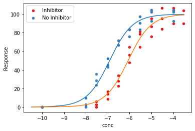
おまけとして図示
def No_inhibitor_theoreticalValue(C):
    Mu=100/(1+10**(prm[0]*(prm[1]-C)))
    return Mu

def Inhibitor_theoreticalValue(C):
    Mu=100/(1+10**(prm[0]*(prm[2]-C)))
    return Mu


fig, ax = plt.subplots()
cmap = plt.get_cmap('Set1')
x1 = np.arange(-10.5, -3.5, 0.01)
for i, (key, df) in enumerate(dat_rec3.groupby('Group')):
    df.plot.scatter(x='conc', y='Response',
    ax=ax, color=cmap(i), label=key, s=20)
ax.plot(x1,No_inhibitor_theoreticalValue(x1))
ax.plot(x1,Inhibitor_theoreticalValue(x1))
ax.legend()
plt.show()
Julia
やっていることはPyhonと殆ど一緒
using Pkg,Optim
using DataFrames,Plots,CSV
using RCall
using LinearAlgebra
using Distributions, Rmath
using Roots
#データの読み込み
#Juliaでデータの前処理がやりづらかったため、前もってRで前処理しておいたデータを読み込み

df=CSV.read("データのパス",DataFrame)
dat_r2=rcopy(R"
G1<-as.numeric(factor($df$Group,levels=unique($df$Group)))-1
G2<-(-1)*(as.numeric(factor($df$Group,levels=unique($df$Group)))-2)
dat_r2<-data.frame(cbind($df,G_1=G1,G_2=G2))
"
)
dat_r3=dat_r2[:,2:7]
#引数をベクトル化

Conc=dat_r3[:,1]
Response=dat_r3[:,2]
G1=dat_r3[:,5]
G2=dat_r3[:,6]

#初期値
p_init=[0.000,-8.000,-9.000]

#上限、下限を定義
p_1=[1.000,-4.000,-4.500]
p_0=[0.000,-8.000,-9.000]


#関数を定義

#用量反応関数を定義
function fun_y(β,x1,x2,x3)
    z=100/(1.0+10^(β[1]*(β[2]*x1+β[3]*x2-x3)))
end

#残差平方和関数を定義

function sqerror(β)
    error=0.0
    for i in  1:length(Conc)
        pred_i=fun_y(β,G1[i],G2[i],Conc[i])
        error +=(Response[i]-pred_i)^2
    end
    return error
end
#パラメータ推定
res=optimize(sqerror,p_init,p_1,p_0)

#パラメータ
parm=res.minimizer
print(parm)

#残差平方和
res_m=res.minimum
print(res_m)
#Parameter
#[Hill,Inhibitor,No Inhibitor]
[0.8298884179757895, -6.068257128529053, -6.913318224632682]

#残差平方和
2056.0386814841204
標準誤差から信頼区間を求める(Julia)
数式では
まず、Response $y_j$と用量反応曲線の関数$f(x_j,\beta)(x_j:Concentration,\beta:parameter)$
の誤差$\epsilon_j$は
$$
\epsilon_j=y_j-f(x_j,\beta)\
$$
の関係式で表すことが出来る。
そして、非線形回帰モデルでは分散共分散行列を
$$
f(x_j,\beta)\simeq f(x_j,\hat \beta)+\nabla f(x_j,\hat \beta)(\beta-\hat \beta) \
$$
$\epsilon:誤差$、$\nabla:f(x_j,\beta)の勾配$
で計算している。
ここで、
$$
g_j=\nabla f(x_j,\hat \beta)
$$
$$
z_j=y_j-f(x_j,\hat \beta)+\nabla f(x_j,\hat \beta)\hat \beta \space
$$
とおき、一番上の$\epsilon$の式に$x_j$の式を代入すると
z_j=g_j \beta+\epsilon_j\\
と変形できる。
そして、これをまとめると
$$
z=G\beta+ \epsilon (行列Gのg_j行目)
$$
と表すことが出来る。
そして証明は省略するがパラメータの推定値$\tilde{\beta}$は
\begin{align}
\tilde{\beta}&=\mathop{\rm arg}\mathop{\rm min}_{\beta}||z-G\beta||^2\\
&=(G′G)^{−1}G′z \\
&=(G′G)^{−1}G′(y-f(x,\hat \beta)+\nabla f(x,\hat \beta)\hat \beta) \\
&=\hat\beta+(G′G)^{-1}\nabla f(x,\hat \beta)(y−f(x,\hat\beta))
\end{align}
であり、分散共分散行列は
$$
\hat\beta=(G′G)^{−1}G′z
$$
より
$$
Var_{lin}(\beta)=\hat \sigma^2 (G′G)^{-1}
$$
(恐らくここら辺の行列表現は永田・棟近がわかりやすいと思う。)
今回もこれを実装する。
実装
各xにおける勾配ベクトルを求める関数を見つけることが出来なかったので(追記の「FowardDiffを用いた標準誤差を求める方法」で書きました)、中心差分法を用いて算出する関数を実装した。
$$
Hill=\frac{\frac{100}{1+10^{((hill+1/2h)(Cont\times EC_{50_{Cont}}-Conc+Group\times EC_{50_{Treat}})}}-\frac{100}{1+10^{(hill-1/2h)(Cont\times EC_{50_{Cont}}-Conc+Group\times EC_{50_{Treat}})}}}{h}
$$
function β1(β,h)
        tmp=(100 ./(1.0 .+10 .^((β[1]+h/2) .*(β[2] .*G1 .+β[3] .*G2 .-Conc))).-
       100 ./(1.0 .+10 .^((β[1]-h/2) .*(β[2] .*G1 .+β[3] .*G2 .-Conc))))/h
end

function β2(β,h)
        tmp=(100 ./(1.0 .+10 .^(β[1].*((β[2]+h/2) .*G1 .+β[3] .*G2 .-Conc))).-
       100 ./(1.0 .+10 .^(β[1] .*((β[2]-h/2) .*G1 .+β[3] .*G2 .-Conc))))/h
end

function β3(β,h)
        tmp=(100 ./(1.0 .+10 .^(β[1].*(β[2] .*G1 .+(β[3]+h/2) .*G2 .-Conc))).-
       100 ./(1.0 .+10 .^(β[1] .*(β[2] .*G1 .+(β[3]-h/2) .*G2 .-Conc))))/h
end

function tmp(β,h)
    tmp=hcat(β1(β,h),β2(β,h),β3(β,h))
    return tmp
end
#刻み幅
h=0.0001

#勾配ベクトルを求める
grad_m=tmp(parm,h)

#ヘッセ行列を求める
hessian=transpose(grad_m)*grad_m


#標準誤差を求める
SE=(diag(inv(hessian))*res_m/(length(Conc)-length(parm))).^(1/2)

#結果を格納
result_lower,result,result_upper=[parm.-SE.*qt(0.975,df),parm,parm.+SE.*qt(0.975,df)]

dat_res=rcopy(R"""
    dat_res<-data.frame($result_lower,$result,$result_upper)
    """
    )

dat_res=rename!(dat_res, [:Lower, :Est, :Upper])
print(dat_res)
 3×3 DataFrame
 Row │ Lower      Est        Upper
     │ Float64    Float64    Float64
─────┼─────────────────────────────────
   1 │  0.736783   0.829888   0.922994
   2 │ -6.15883   -6.06826   -5.97768
   3 │ -7.00428   -6.91332   -6.82236
FowardDiffを用いた標準誤差を求める方法(追記(24th,Aug,2022))
黒木玄先生から、Juliaの「標準誤差から信頼区間を求める(Julia)」のところでForwardDiff.jlのgradientが使えるのではと指摘があった。
そこで、
を参考にForwardDiff.jlを試すことにした。
(実は昔ForwardDiffのgradientを試したことがあったのだが、複数パラメータで上手くいかなかったため断念した経緯がある。)
ipynbファイルの1つめのセルの13~18行目の
"""ϕ should be a potential function."""
function LFProblem(dim, ϕ; dt = 1.0, nsteps = 40)
    H(x, v, param) = dot(v, v)/2 + ϕ(x, param)
    F(x, param) = -gradient(x -> ϕ(x, param), x)
    LFProblem{dim}(ϕ, H, F, dt, nsteps)
end
の部分を参考に
using ForwardDiff
using Flux

β_param=β_param=hcat(collect.(parm)...)

tmp_4=[]
for i in 1:length(Conc)
    tmp_3=[]
    tmp_3=gradient(y->fun_y(y,G1[i],G2[i],Conc[i]),β_param)
    tmp_4=vcat(tmp_4,tmp_3)
end
と書いた。
特に、
tmp_3=gradient(y->fun_y(y,G1[i],G2[i],Conc[i]),β_param)
の書き方をすれば、複数のパラメータを引数にとって実行できる。
上記のコードを実行すると、
tmp4

56-element Vector{Any}:
 ([-1.939661153344207 0.0 -0.5214992808147069],)
 ([-24.76890747396581 0.0 -18.91577636112475],)
 ([-25.441435626656858 0.0 -34.63044758147603],)
 ([-4.955734486104251 0.0 -47.44603620718794],)
 ([19.612153788088108 0.0 -41.699050295719964],)
 ([26.613656628829226 0.0 -24.1825519304979],)
 ([19.615987838260533 0.0 -11.708888530485348],)
 ([10.81458131494866 0.0 -4.690749120030085],)
 ([2.544258845078717 0.0 -0.7247580885639441],)
 ([-1.939661153344207 0.0 -0.5214992808147069],)
 ([-24.76890747396581 0.0 -18.91577636112475],)
 ([-25.441435626656858 0.0 -34.63044758147603],)
 ([-4.955734486104251 0.0 -47.44603620718794],)
 ⋮
 ([16.773935051380214 -9.00852949713918 0.0],)
 ([8.807818265847034 -3.534138123174552 0.0],)
 ([4.456424987549471 -1.4530302032323696 0.0],)
 ([-0.49364974248449867 -0.10419659098188912 0.0],)
 ([-18.42636266625523 -10.511702969669512 0.0],)
 ([-26.482945838891958 -23.587934717310976 0.0],)
 ([-21.79689220119996 -39.77849796112387 0.0],)
 ([3.9125321240294793 -47.56961162390871 0.0],)
 ([24.202683635101298 -36.83679824028657 0.0],)
 ([25.021319758713325 -19.43811364855332 0.0],)
 ([16.773935051380214 -9.00852949713918 0.0],)
 ([8.807818265847034 -3.534138123174552 0.0],)
となる。
これを下記の記事を参考にtmp_4をMatrixデータに変換する。
tmp_5=vcat(collect.(tmp_4)...)

56-element Vector{Matrix{Float64}}:
 [-1.939661153344207 0.0 -0.5214992808147069]
 [-24.76890747396581 0.0 -18.91577636112475]
 [-25.441435626656858 0.0 -34.63044758147603]
 [-4.955734486104251 0.0 -47.44603620718794]
 [19.612153788088108 0.0 -41.699050295719964]
 [26.613656628829226 0.0 -24.1825519304979]
 [19.615987838260533 0.0 -11.708888530485348]
 [10.81458131494866 0.0 -4.690749120030085]
 [2.544258845078717 0.0 -0.7247580885639441]
 [-1.939661153344207 0.0 -0.5214992808147069]
 [-24.76890747396581 0.0 -18.91577636112475]
 [-25.441435626656858 0.0 -34.63044758147603]
 [-4.955734486104251 0.0 -47.44603620718794]
 ⋮
 [16.773935051380214 -9.00852949713918 0.0]
 [8.807818265847034 -3.534138123174552 0.0]
 [4.456424987549471 -1.4530302032323696 0.0]
 [-0.49364974248449867 -0.10419659098188912 0.0]
 [-18.42636266625523 -10.511702969669512 0.0]
 [-26.482945838891958 -23.587934717310976 0.0]
 [-21.79689220119996 -39.77849796112387 0.0]
 [3.9125321240294793 -47.56961162390871 0.0]
 [24.202683635101298 -36.83679824028657 0.0]
 [25.021319758713325 -19.43811364855332 0.0]
 [16.773935051380214 -9.00852949713918 0.0]
 [8.807818265847034 -3.534138123174552 0.0]
このtmp_5は上記のgrad_mと等しい。
その証拠に、tmp_5を転置した行列とtmp_5そのものをかけ算を実行し、その結果を比較する。
hessian_grad=transpose(tmp_5)*tmp_5

3×3 Matrix{Float64}:
 18017.3     -195.354   -473.806
  -195.354  19025.8        0.0
  -473.806      0.0    18875.1
hessian

3×3 Matrix{Float64}:
 18017.3     -195.354   -473.806
  -195.354  19025.8        0.0
  -473.806      0.0    18875.1
そのため上記の標準誤差から信頼区間を出力するまでの手順は
# Dose Response Function
function fun_y(β,x1,x2,x3)
    z=100/(1.0+10^(β[1]*(β[2]*x1+β[3]*x2-x3)))
end

# Function for Nonlinear Least Squares

function resp_1(β,x1,x2,x3,x4)
    error=0.0
    for i in  1:length(x4)
        pred_i=fun_y(β,x1[i],x2[i],x3[i])
        error +=(x4[i]-pred_i)^2
    end
    return error
end

# Function for find the Hessian

function hessian_1(β,x1,x2,x3)
    tmp2=[]
    for i in 1:length(x1)
    tmp=gradient(y->fun_y(y,x1[i],x2[i],x3[i]),β)
    tmp2=vcat(tmp2,tmp)
    end
    tmp3=vcat(collect.(tmp2)...)
    hes=transpose(tmp3)*tmp3
    return hes
end

# Function for find Standard Error


function SEroor(β,x1,x2,x3,Res)
    #SE=(diag(inv(hessian))*res_m/(length(Conc)-length(parm))).^(1/2)
    hes=hessian_1(β,x1,x2,x3)
    df=length(x3)-length(β)
    SE=diag(inv(hes))*Res/df
    return SE
end
とまとめることができる。
ここまで来れば、
result_lower,result,result_upper=[parm.-SE.*qt(0.975,df),parm,parm.+SE.*qt(0.975,df)]
で信頼区間を求めることが出来る。
Profile Likelyhood(Julia)
やっていることはPythonと同じ。
#各Profile Likelyhoodを求めるための用量反応関数を定義

function fun_y2(β1,x1,x2,x3)
    z=100/(1.0+10^(β1*(parm[2]*x1+parm[3]*x2-x3)))
end

function fun_y3(β2,x1,x2,x3)
    z=100/(1.0+10^(parm[1]*(β2*x1+parm[3]*x2-x3)))
end

function fun_y4(β3,x1,x2,x3)
    z=100/(1.0+10^(parm[1]*(parm[2]*x1+β3*x2-x3)))
end


function sqerror2(β1)
    error=0.0
    error1=0.0
    for i in  1:length(Conc)
        pred_i=fun_y2(β1,G1[i],G2[i],Conc[i])
        error +=(Response[i]-pred_i)^2
    end
    error1=error-(qf(0.95,1,df)/df+1)*res_m
    return error1
end


function sqerror3(β2)
    error=0.0
    error1=0.0
    for i in  1:length(Conc)
        pred_i=fun_y3(β2,G1[i],G2[i],Conc[i])
        error +=(Response[i]-pred_i)^2
    end
    error1=error-(qf(0.95,1,df)/df+1)*res_m
    return error1
end


function sqerror4(β3)
    error=0.0
    error1=0.0
    for i in  1:length(Conc)
        pred_i=fun_y4(β3,G1[i],G2[i],Conc[i])
        error +=(Response[i]-pred_i)^2
    end
    error1=error-(qf(0.95,1,df)/df+1)*res_m
    return error1
end


#各Profile Likelyhoodを求めるための用量反応関数を定義

#Hill係数
function sqerror2(β1)
    error=0.0
    error1=0.0
    for i in  1:length(Conc)
        pred_i=fun_y2(β1,G1[i],G2[i],Conc[i])
        error +=(Response[i]-pred_i)^2
    end
    error1=error-(qf(0.95,1,df)/df+1)*res_m
    return error1
end


#Treat EC50

function sqerror3(β2)
    error=0.0
    error1=0.0
    for i in  1:length(Conc)
        pred_i=fun_y3(β2,G1[i],G2[i],Conc[i])
        error +=(Response[i]-pred_i)^2
    end
    error1=error-(qf(0.95,1,df)/df+1)*res_m
    return error1
end

#Non Treat EC50

function sqerror4(β3)
    error=0.0
    error1=0.0
    for i in  1:length(Conc)
        pred_i=fun_y4(β3,G1[i],G2[i],Conc[i])
        error +=(Response[i]-pred_i)^2
    end
    error1=error-(qf(0.95,1,df)/df+1)*res_m
    return error1
end
#Hill係数の信頼区間

hill_low,hill,hill_upp=[Roots.find_zero(sqerror2,0),parm[1],Roots.find_zero(sqerror2,1)]


#Treat群のEC50の信頼区間

Treat_low,Treat,Treat_upp=[Roots.find_zero(sqerror3,-7.5),parm[2],Roots.find_zero(sqerror3,-5)]

#Non Treat群のEC50の信頼区間
Non_low,Non,Non_upp=[Roots.find_zero(sqerror4,-7.5),parm[3],Roots.find_zero(sqerror4,-5)]

Lower=[hill_low,Treat_low,Non_low]
Upper=[hill_upp,Treat_upp,Treat_upp]

#Dataframeに格納

dat_res2=rcopy(R"""
    dat_res<-data.frame($Lower,$parm,$Upper)
    """
    )
dat_res2=rename!(dat_res2, [:Lower, :Est, :Upper])


print(dat_res2)
3×3 DataFrame
 Row │ Lower      Est        Upper
     │ Float64    Float64    Float64
─────┼─────────────────────────────────
   1 │  0.744566   0.829888   0.928687
   2 │ -6.15792   -6.06826   -5.97853
   3 │ -7.00547   -6.91332   -5.97853
最後に
次は、Stanを用いた推定かLevenberg-Marquardt法をフルスクラッチする記事かなと思います。
参考文献
ガルバッタ氏のブログ
用量反応曲線のEC50の標準偏差を出す
Nonlinear regression
http://sia.webpopix.org/nonlinearRegression.html
(22th,Apr,2022:追記 リンク先に飛ぶと詐欺サイトに飛ぶ可能性が出たため、以下のアーカイブに)
多変量解析法入門
永田 靖、棟近雅彦
第2期 医薬安全性研究会
非線形最小2乗法の基礎
(1) 線形モデルと非線形モデルの基本的な考え方
逆推定の解析,標準誤差と信頼限界 大和田 章一
最小2乗法,最尤法 線形モデル,非線形モデル 芳賀 敏郎