tf.function の使い方について #TensorFlow

この記事では TensorFlow 2.0 で導入された tf.function について、概要を取り扱います。

TL;DR

tf.function は Eager Execution の書きやすさと、 1.x 系列の性能とを両立させるものです
Python の関数を @tf.function でデコレートすることにより、TensorFlow のグラフへとコンパイルし最適化できます
@tf.function でデコレートした関数は AutoGraph により、自動微分ができるようになります
tf.function を前処理に使ってみたところ、10倍程度の高速化ができました

背景

tf.function は TensorFlow 2.x 系で導入された新たな機能で、これにより機械学習に用いられる計算グラフをより見通しよく記述することができます。ここでは tf.function の解決したい課題について見てみましょう。

TensorFlow における tf.function の提案は Functions, not sessions でなされました。ここでは次の事項を目的に掲げています。

Encourage the encapsulation of graph computation as Python functions (where the graph is executed when the function is invoked, instead of via Session)

Align "state" in the TensorFlow runtime (e.g., resource tensors like those that back tf.Variable objects) with state in the Python program (e.g., Python objects corresponding to the runtime state with lifetimes attached to each other).

Make it easy to export these encapsulations to a GraphDef+Checkpoint and/or SavedModel.

Enable eager execution by default.

Provide a path for incorporating existing code that uses the 1.x APIs to construct TensorFlows graphs as functions in TensorFlow 2.x programs.

それぞれ翻訳すると次のようになります。

計算 Graph の実行をし、 Python の関数のようにカプセル化する (計算グラフは Session 内ではなく、関数が呼ばれたときに実行される)

TensorFlow における "状態" (e.g., tf.Variable オブジェクトで使われる resource tensors) を Python のプログラムにおける "状態" (e.g., 実行中のランタイムの状態を表す Python のオブジェクト) のようにする

GraphDef + Checkpoint や SavedModel への出力をカプセル化し、簡単にできるようにする

Eager execution をデフォルトで有効にする

現在存在する 1.x 系 API を利用しているコードから、TensorFlow 2.x 系で Graph を関数として利用するプログラムを構築するための道筋を示す

TensorFlow 2.x 系では Eager Execution がデフォルトで有効になり、Keras を用いた場合のコードの見た目が他の深層学習フレームワークに近づきました。 1.x 系列の Session を用いたコードを、2.x 系列の tf.function を用いたコードと比較してみましょう。

# TensorFlow 1.x
W = tf.Variable(
  tf.glorot_uniform_initializer()(
    (10, 10)))
b = tf.Variable(tf.zeros(10))
c = tf.Variable(0)

x = tf.placeholder(tf.float32)
ctr = c.assign_add(1)
with tf.control_dependencies([ctr]):
  y = tf.matmul(x, W) + b
init = 
  tf.global_variables_initializer()

with tf.Session() as sess:
  sess.run(init)
  print(sess.run(y,
  feed_dict={x: make_input_value()}))
  assert int(sess.run(c)) == 1

同様のコードを tf.function を用いて記述すると次のようになります。

# TensorFlow 2.x
W = tf.Variable(
  tf.glorot_uniform_initializer()(
    (10, 10)))
b = tf.Variable(tf.zeros(10))
c = tf.Variable(0)

@tf.function
def f(x):
  c.assign_add(1)
  return tf.matmul(x, W) + b

print(f(make_input_value())
assert int(c) == 1

2.x系では Python における通常の関数呼び出しのように、スッキリと書けるようになったことがわかります。

`tf.function` の使い方

ここでは tf.function の基本的な使い方について記します。

まずは最もかんたんな例を確認しましょう。tf.function はデコレーターとして @tf.funciton を用いることで利用できます。

# A function is like an op

@tf.function
def add(a, b):
  return a + b

add(1, 1) # <tf.Tensor: id=19, shape=(), dtype=int32, numpy=2>

通常のPythonの関数と異なり tf.Tensor が帰ってきているのが分かります。実際に帰ってきた値を得るためには次のようにします。

result = add(1, 1)
result.numpy() # 2

このように、@tf.function を適用した関数は tf.Tensor を出力するようになります。入力には Python の組み込み型以外にも Numpy の配列を渡すこともできます。

import numpy as np
add(np.ones(2), np.ones(2)) # <tf.Tensor: id=38, shape=(2,), dtype=float64, numpy=array([2., 2.])>

もちろん、tf.Tensor を渡すこともできます。

add(tf.constant(1), tf.constant(1)) # <tf.Tensor: id=47, shape=(), dtype=int32, numpy=2>

このように、tf.function を用いると tf.Tensor を入出力する関数を通常の Python の関数を定義するように記述できます。また、Eager Execution により、その利用もあたかも通常の Python の関数であるかのように行われます。

次に高速化について検討します。@tf.function を適用した関数は、引数の型を指定して Graph にコンパイルできます。

add_int = add.get_concrete_function(
     tf.TensorSpec(shape=None, dtype=tf.int32), 
     tf.TensorSpec(shape=None, dtype=tf.int32)
)
add_int(tf.constant(2), tf.constant(2)) # 2

これにより計算が高速化されることが期待できます (今回の場合は計算量が軽微なためあまり目立った差は見られません)。

# On Jupyter Notebook
%timeit add(tf.constant(2), tf.constant(2)) # 1000 loops, best of 3: 277 µs per loop
%timeit add_int(tf.constant(2), tf.constant(2)) # 1000 loops, best of 3: 196 µs per loop

生成された計算グラフは次のようにすると確認できます。

add_int.function_def

出力は次のようになります。長いので中略しましたが、引数の型が指定され、続いて定義した関数について記述されていることが分かります。

signature {
  name: "__inference_add_101"
  input_arg {
    name: "a"
    type: DT_INT32
  }
  input_arg {
    name: "b"
    type: DT_INT32
  }
  output_arg {
    name: "identity"
    type: DT_INT32
  }
}
node_def {
  name: "add"
  op: "AddV2"
  input: "a"
  input: "b"
  attr {
    key: "T"
    value {
      type: DT_INT32
    }
  }
}
  :
  :
arg_attr {
  key: 1
  value {
    attr {
      key: "_user_specified_name"
      value {
        s: "b"
      }
    }
  }
}

以上のように、tf.fuction を用いることで 2.x 系の特徴である書きやすさと、 1.x 系の特徴であるコンパイルによる実行速度の向上の両立が実現されます。

最後にデバッグについて見てみましょう。@tf.function を用いて修飾した関数について、デフォルトではステップ実行するデバッガー (例えば pdb)をサポートしていませんが、tf.config.run_functions_eagerly(True) を有効にすることで、対話型のデバッガーの利用が可能になります。

@tf.function
def f(x):
  if x > 0:
    # Try setting a breakpoint here!
    # Example:
    import pdb
    pdb.set_trace()
    x = x + 1
  return x

tf.config.experimental_run_functions_eagerly(True)

# You can now set breakpoints and run the code in a debugger.
f(tf.constant(1))

Colab上で上記のコードを実行している様子がこちらです。

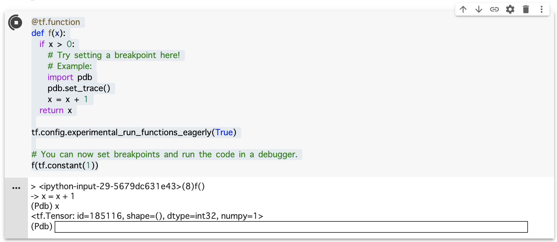
対話型のデバッグができていることと、実行中の変数が参照できていることが分かります。今までは専用のデバッガーが必要でしたが、これからは自分の好きなデバッガを用いることができるようになります (experimental である点には注意が必要ですが)。

AutoGraph を利用した自動微分

tf.function を適用すると、その関数について勾配を計算できるようになります。ここでも最も単純な例で動作を確認しましょう。

@tf.function
def identity(x):
  return x

v = tf.Variable(5.0)
with tf.GradientTape() as tape:
  result = identity(v)
tape.gradient(result, v) # <tf.Tensor: id=185192, shape=(), dtype=float32, numpy=1.0>

tf.GradientTape を呼び出すことで、以降で行われた計算の記録が行われます。ここでは $$y = x$$ に相当する計算が行われています。これを微分した結果は $$y' = 1$$ ですので、結果は1になります。正しく微分が計算できていることが分かります。

勾配の計算について、ここで詳細を述べることはしませんが、1変数だけでなく多変数の微分を行うことも可能です。Better performance with tf.function から該当の箇所を抜粋します。

# You can use functions inside functions

@tf.function
def dense_layer(x, w, b):
  return add(tf.matmul(x, w), b)

dense_layer(tf.ones([3, 2]), tf.ones([2, 2]), tf.ones([2]))
# <tf.Tensor: id=185218, shape=(3, 2), dtype=float32, numpy=
# array([[3., 3.],
#        [3., 3.],
#        [3., 3.]], dtype=float32)>

実験: 前処理への適用

ここまでで、ごく単純な例を用いて tf.funciton の機能を確認してきましたが、より実例に近い処理に適用してみましょう。ここでは、tf.data: Build TensorFlow input pipelines にある画像をランダムな角度だけ回転させる処理を行ってみます。これは画像を学習用データとして用いる場合に前処理として行われる典型的な処理の一つです。

tf.function を使わない場合の実装は例えば次のようになるでしょう。

def reshape_fn(image):
  return tf.reshape(image, (28, 28, 1))

def rotate_fn(image):
  return ndimage.rotate(image, np.random.uniform(-30, 30), reshape=False)

def tf_reshape(image):
  reshaped = tf.py_function(reshape_fn, [image], [tf.uint8])
  return reshaped[0]

def tf_rotate(image):
  rotated = tf.py_function(rotate_fn,[image],[tf.uint8])
  return rotated[0]

def preprocess_without_tf_funciton(dataset):
  return dataset.map(tf_reshape).map(tf_rotate).batch(16)

(train_x, train_y), (test_x, test_y) =  keras.datasets.mnist.load_data()
train_ds = tf.data.Dataset.from_tensor_slices(train_x)

batched_train_ds = preprocess_without_tf_funciton(train_ds)

同様の処理を tf.function を用いて記述すると次のようになります。変更点は @tf.function でデコレートしたことのみです。

@tf.function
def preprocess_with_tf_funciton(dataset):
  return dataset.map(tf_reshape).map(tf_rotate).batch(16)

batched_train_ds = preprocess_with_tf_funciton(train_ds)

実行層度を%%timeitを用いて比較したところ、tf.function を用いない場合の実行速度は 6.45 ms per loop でした。一方、tf.function を用いた場合には best of 3: 416 µs per loop とおおよそ 10 倍程度高速化できました。

実装の全体については better performance with tf.function.ipynb を参照ください。Colab へのリンクもあるので、手元で確認することもできます。

最後に

tf.function を用いれば問題がすべて解決するかと言うとそういうわけではありません。

ごく単純な演算において実行速度を向上することが必ずしもできない点は見てきましたが、その他にも Retracing に関して自明でない振る舞いをする場合があり、こちらも注意が必要です。詳細は Better performance with tf.function and AutoGraph #re-tracing を参照ください。

また、AutoGraph による自動微分を行うためには、記法に制約が加わる点にも注意が必要でしょう。例えば、変数への再代入は推奨されませんし、関数内の副作用についても推奨されません。詳細はtensorflow/limitationsを参照ください。

ですが、tf.function により機械学習モデルをより柔軟に、より高速に実行できるようになったことは事実です。例えば、 Convolutional Variational Autoencoder のチュートリアルではtf.function と AutoGraph を用いて学習処理を記述することで、中間層の出力結果を用いた学習を可能にしています。

tf.function は既存のモデルの枠組みを踏み越えて、独自のモデルを記述する場合に役に立つことが期待できると筆者は考えます。

tf.function の使い方について

TL;DR

背景

tf.function の使い方

AutoGraph を利用した自動微分

実験: 前処理への適用

最後に

Reference

`tf.function` の使い方