少し前にkaggleのkernelから時系列を勉強していたのですが、outputが自分の想像していたようなものではなく満足できなかったので
時系列データのモデリングに関して少し追いかけてみたいと思いました。
手を動かしてみる
データは引き続きこちらを使います。
weather_station_location = pd.read_csv('Weather Station Locations.csv')
weather = pd.read_csv("Summary of Weather.csv")

weather_station_location = weather_station_location.loc[:,["WBAN","NAME","STATE/COUNTRY ID","Latitude","Longitude"] ]
weather_station_location.info()

weather_station_id = weather_station_location[weather_station_location.NAME == "BINDUKURI"].WBAN
weather_bin = weather[weather.STA == 32907]
weather_bin["Date"] = pd.to_datetime(weather_bin["Date"])

plt.figure(figsize=(22,10))
plt.plot(weather_bin.Date,weather_bin.MeanTemp)
plt.title("Mean Temperature of Bindukuri Area")
plt.xlabel("Date")
plt.ylabel("Mean Temperature")
plt.show()
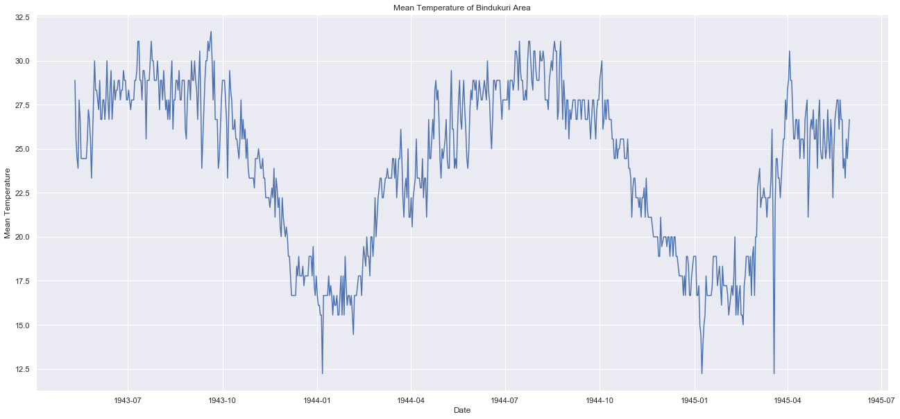
まずplotしましょう。
t1=weather_bin.Date
t2=weather_bin.MeanTemp
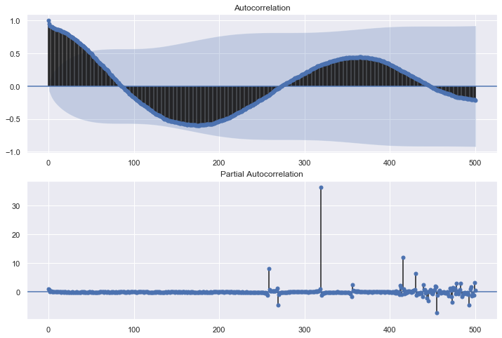
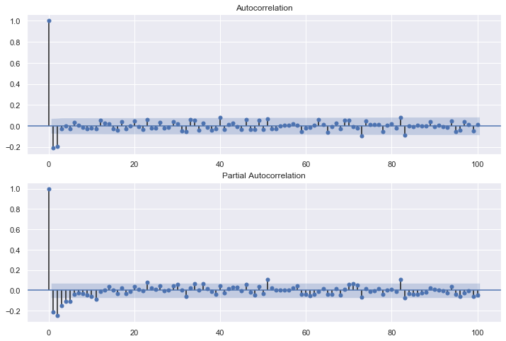
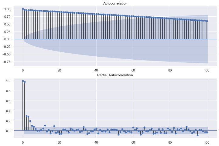
ts_acf = sm.tsa.stattools.acf(t2, nlags=500)
fig = plt.figure(figsize=(12,8))
ax1 = fig.add_subplot(211)
fig = sm.graphics.tsa.plot_acf(t2, lags=500, ax=ax1)
ax2 = fig.add_subplot(212)
fig = sm.graphics.tsa.plot_pacf(t2, lags=500, ax=ax2)
元のデータを見ると1945年4月に寒波?のようなものが観測されている。
acfは定常波。
pacfは300を少し超えたところで影響が出ている。
ここでネットを見ていると時系列分析している方がいたので参考にさせてもらうことに。
こちら!→ logics of blue
この方のPythonで学ぶあたらしい統計学の教科書はpythonも統計も始めたばかりの頃読みましたが大変わかりやすく書かれておりました。新しくstanの本も書かれているので是非読んでみたいと思います。
とっととモデル作ろうや
mod = sm.tsa.statespace.SARIMAX(t2, trend='n', order=(1,0,50), seasonal_order=(0,0,0,12))
results = mod.fit()
print (results.summary())
まず最初にこんなモデルを作ってみました。
seasonal_orderのsには周期性を入れるのですが、とりあえず12か月あるし12かな?とか勘違いして12って入れています。
(実際には1日づつのデータなので360で一周なのですが。。。)
結果は
                           Statespace Model Results
==============================================================================
Dep. Variable:               MeanTemp   No. Observations:                  751
Model:              SARIMAX(1, 0, 50)   Log Likelihood               -1250.845
Date:                Tue, 09 Jul 2019   AIC                           2605.691
Time:                        18:29:37   BIC                           2846.004
Sample:                             0   HQIC                          2698.283
                                - 751
Covariance Type:                  opg
==============================================================================
                 coef    std err          z      P>|z|      [0.025      0.975]
------------------------------------------------------------------------------
ar.L1          0.9994      0.001   1163.196      0.000       0.998       1.001
ma.L1         -0.3505      0.029    -12.090      0.000      -0.407      -0.294
ma.L2         -0.2456      0.036     -6.779      0.000      -0.317      -0.175
ma.L3         -0.0449      0.037     -1.219      0.223      -0.117       0.027
ma.L4          0.0115      0.043      0.266      0.791      -0.073       0.097
ma.L5         -0.0224      0.046     -0.488      0.626      -0.112       0.068
ma.L6          0.0017      0.048      0.035      0.972      -0.092       0.095
ma.L7         -0.0188      0.050     -0.377      0.706      -0.116       0.079
ma.L8         -0.0136      0.046     -0.295      0.768      -0.104       0.077
ma.L9         -0.0400      0.044     -0.901      0.368      -0.127       0.047
ma.L10        -0.0037      0.046     -0.080      0.936      -0.094       0.087
ma.L11        -0.0044      0.040     -0.108      0.914      -0.084       0.075
ma.L12         0.0864      0.043      2.027      0.043       0.003       0.170
ma.L13         0.0310      0.039      0.800      0.424      -0.045       0.107
ma.L14         0.0008      0.041      0.020      0.984      -0.080       0.081
ma.L15        -0.0488      0.039     -1.247      0.212      -0.125       0.028
ma.L16        -0.0242      0.040     -0.598      0.550      -0.103       0.055
ma.L17         0.0404      0.043      0.928      0.353      -0.045       0.126
ma.L18        -0.0076      0.043     -0.176      0.860      -0.092       0.077
ma.L19         0.0692      0.041      1.674      0.094      -0.012       0.150
ma.L20         0.0258      0.043      0.605      0.545      -0.058       0.109
ma.L21        -0.0593      0.046     -1.298      0.194      -0.149       0.030
ma.L22        -0.0087      0.045     -0.192      0.848      -0.097       0.080
ma.L23         0.0559      0.049      1.139      0.255      -0.040       0.152
ma.L24        -0.0195      0.046     -0.424      0.671      -0.110       0.071
ma.L25         0.0040      0.040      0.101      0.920      -0.075       0.083
ma.L26         0.0569      0.047      1.211      0.226      -0.035       0.149
ma.L27        -0.0360      0.042     -0.862      0.389      -0.118       0.046
ma.L28        -0.0382      0.043     -0.897      0.370      -0.122       0.045
ma.L29         0.0453      0.043      1.045      0.296      -0.040       0.130
ma.L30        -0.0125      0.043     -0.292      0.770      -0.096       0.071
ma.L31        -0.0600      0.046     -1.312      0.189      -0.150       0.030
ma.L32         0.0230      0.043      0.538      0.591      -0.061       0.107
ma.L33         0.1110      0.040      2.809      0.005       0.034       0.188
ma.L34         0.0396      0.049      0.815      0.415      -0.056       0.135
ma.L35        -0.0595      0.045     -1.328      0.184      -0.147       0.028
ma.L36        -0.0111      0.050     -0.223      0.823      -0.109       0.086
ma.L37        -0.0450      0.048     -0.933      0.351      -0.139       0.050
ma.L38        -0.0215      0.046     -0.468      0.640      -0.111       0.068
ma.L39         0.0660      0.048      1.367      0.172      -0.029       0.161
ma.L40         0.0819      0.051      1.612      0.107      -0.018       0.182
ma.L41        -0.0676      0.046     -1.480      0.139      -0.157       0.022
ma.L42         0.0301      0.045      0.668      0.504      -0.058       0.118
ma.L43         0.0260      0.047      0.553      0.580      -0.066       0.118
ma.L44        -0.0271      0.048     -0.564      0.573      -0.121       0.067
ma.L45        -0.0286      0.049     -0.588      0.557      -0.124       0.067
ma.L46         0.0908      0.050      1.803      0.071      -0.008       0.190
ma.L47        -0.0524      0.046     -1.145      0.252      -0.142       0.037
ma.L48        -0.0315      0.047     -0.675      0.500      -0.123       0.060
ma.L49         0.0995      0.044      2.265      0.023       0.013       0.186
ma.L50        -0.0489      0.042     -1.158      0.247      -0.132       0.034
sigma2         1.6185      0.077     21.101      0.000       1.468       1.769
===================================================================================
Ljung-Box (Q):                        3.06   Jarque-Bera (JB):               428.55
Prob(Q):                              1.00   Prob(JB):                         0.00
Heteroskedasticity (H):               1.28   Skew:                            -0.59
Prob(H) (two-sided):                  0.05   Kurtosis:                         6.51
===================================================================================
あー、なるほどね。(わからん)
時系列になってるからわかりにくいのでindexを変えてしまいます。
t3=t2.reset_index()
t3=t3.drop('index',axis=1)
plt.figure(figsize=(22,10))
plt.plot(t3)
plt.title("Mean Temperature of Bindukuri Area")
plt.xlabel("Date")
plt.ylabel("Mean Temperature")
plt.show()
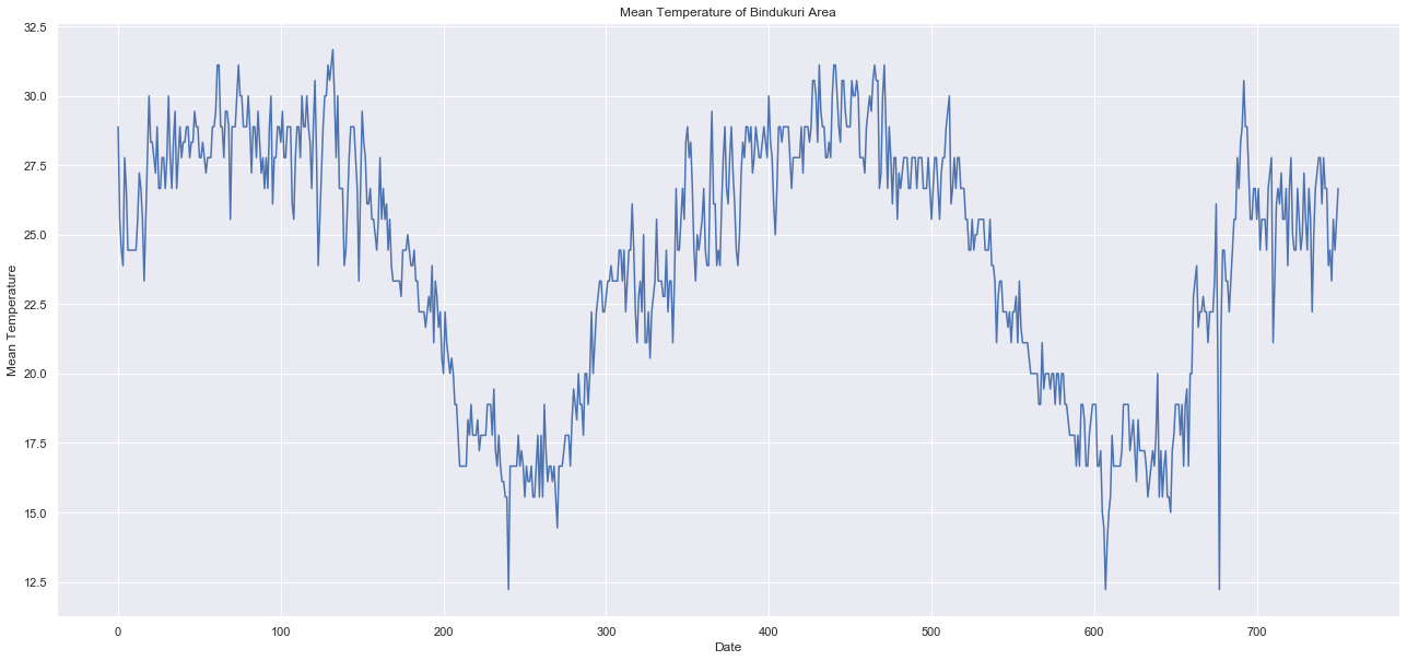
indexを0から始まる数字に変えました。360で一周している季節性が見えました。
元のカーネルはここから定常性になるデータに変換して、AIRMAに入れてモデリングして・・・って感じです。
# adfuller library
from statsmodels.tsa.stattools import adfuller
# check_adfuller
def check_adfuller(t3):
    # Dickey-Fuller test
    result = adfuller(t3, autolag='AIC')
    print('Test statistic: ' , result[0])
    print('p-value: '  ,result[1])
    print('Critical Values:' ,result[4])

# check_mean_std
def check_mean_std(t3):
    #Rolling statistics
    #rolmean = pd.rolling_mean(ts, window=6)
    rolmean = t3.rolling(window=6).mean()
    #rolstd = pd.rolling_std(ts, window=6)
    rolstd = t3.rolling(window=6).std()
    plt.figure(figsize=(22,10))
    orig = plt.plot(t3, color='red',label='Original')
    mean = plt.plot(rolmean, color='black', label='Rolling Mean')
    std = plt.plot(rolstd, color='green', label = 'Rolling Std')
    plt.xlabel("Date")
    plt.ylabel("Mean Temperature")
    plt.title('Rolling Mean & Standard Deviation')
    plt.legend()
    plt.show()

# check stationary: mean, variance(std)and adfuller test
check_mean_std(t3)
check_adfuller(t3.MeanTemp)

# Moving average method
window_size = 6
# moving_avg = pd.rolling_mean(ts,window_size)
moving_avg = t3.rolling(window_size).mean()

plt.figure(figsize=(22,10))
plt.plot(t3, color = "red",label = "Original")
plt.plot(moving_avg, color='black', label = "moving_avg_mean")
plt.title("Mean Temperature of Bindukuri Area")
plt.xlabel("Date")
plt.ylabel("Mean Temperature")
plt.legend()
plt.show()

t3_moving_avg_diff = t3 - moving_avg
t3_moving_avg_diff.dropna(inplace=True)
check_mean_std(t3_moving_avg_diff)
check_adfuller(t3_moving_avg_diff.MeanTemp)

# differencing method
t3_diff = t3 - t3.shift()
plt.figure(figsize=(22,10))
plt.plot(t3_diff)
plt.title("Differencing method")
plt.xlabel("Date")
plt.ylabel("Differencing Mean Temperature")
plt.show()

t3_diff.dropna(inplace=True) # due to shifting there is nan values
# check stationary: mean, variance(std)and adfuller test
check_mean_std(t3_diff)
check_adfuller(t3_diff.MeanTemp)

# ARIMA LİBRARY
from statsmodels.tsa.arima_model import ARIMA
from pandas import datetime

# fit model
model = ARIMA(t3, order=(1,0,1)) # (ARMA) = (1,0,1)
model_fit = model.fit(disp=0)

# predict
start_index = (700)
end_index = (751)
forecast = model_fit.predict(start=start_index, end=end_index)

# visualization
plt.figure(figsize=(22,10))
plt.xlim(745, 755)
plt.plot(t3,label = "original")
plt.plot(forecast,label = "predicted")
plt.title("Time Series Forecast")
plt.xlabel("Date")
plt.ylabel("Mean Temperature")
plt.legend()
plt.show()
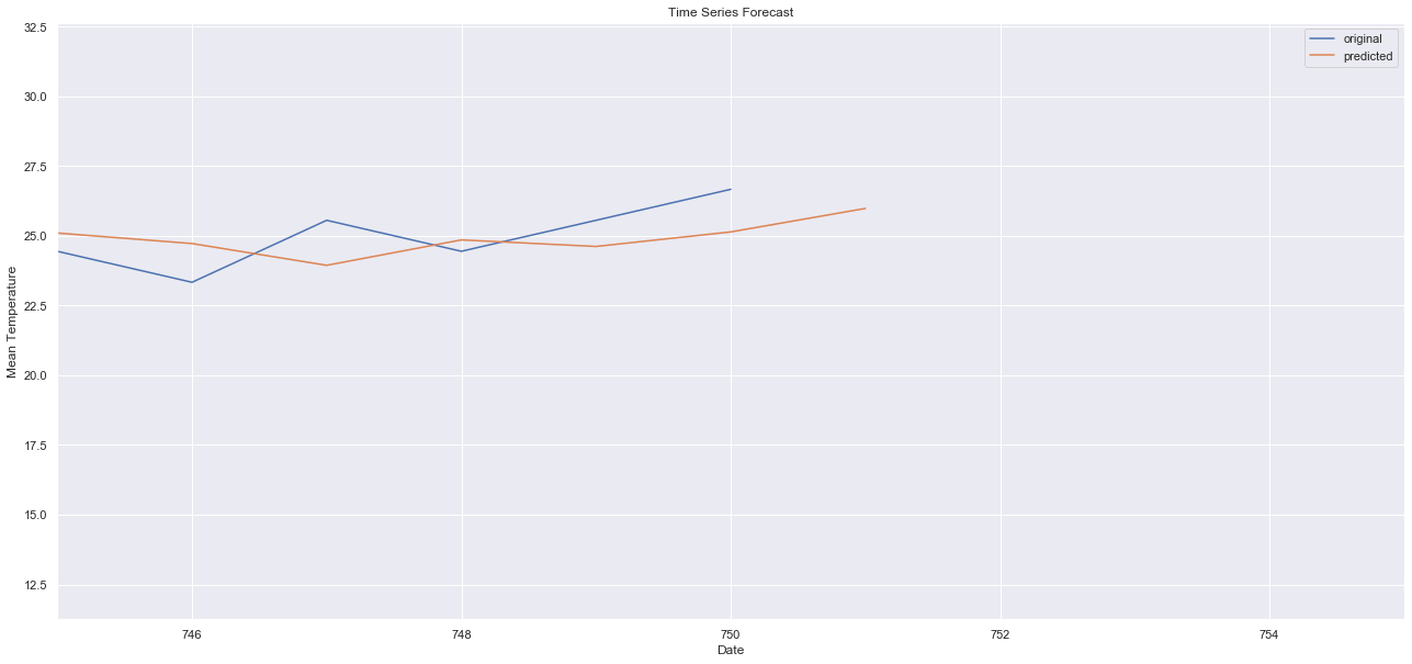
これ以降が予測できてないやんけ!!
ここで不満に思ったわけです。
ちなみにpredictする範囲を未来に設定するとエラーで予測できません。
(なぜなのか誰か教えてください。。。。)
不満解消に向けて動き出す
試行錯誤していきます(これがBox-Jenkins法か???)
ここから上記で紹介させていただいた記事を参考にモデリングしていきます。
コードはデータに合うように改造しています。
SARIMAを使用していますが、パラメータは周期性以外かなり適当です。
他のブログ記事の総当たり法などを実際に組んでみて候補をだしましたがうまくいきませんでした。
以下のうまくいっていない例はその時に候補として出てきたものと、適当に動かしたものが混ざっています。
最終的に少しは納得がいくモデルになるのですが、その時のパラメータの決め方も適当でまぐれです(泣)
1st try
import statsmodels.api as sm
SARIMA_3_1_2_111 = sm.tsa.SARIMAX(t3_diff, order=(0,0,0), seasonal_order=(0,0,0,300)).fit()
print(SARIMA_3_1_2_111.summary())
residSARIMA = SARIMA_3_1_2_111.resid
fig = plt.figure(figsize=(12,8))
ax1 = fig.add_subplot(211)
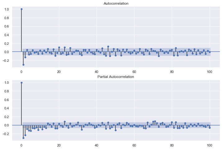
fig = sm.graphics.tsa.plot_acf(residSARIMA.values.squeeze(), lags=100, ax=ax1)
ax2 = fig.add_subplot(212)
fig = sm.graphics.tsa.plot_pacf(residSARIMA, lags=100, ax=ax2)
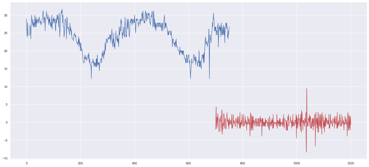
pred = SARIMA_0_0_0_000.predict(700, 1200)
plt.figure(figsize=(22,10))
plt.plot(t3)
plt.plot(pred, "r")
                           Statespace Model Results
==============================================================================
Dep. Variable:               MeanTemp   No. Observations:                  750
Model:                        SARIMAX   Log Likelihood               -1331.318
Date:                Tue, 09 Jul 2019   AIC                           2664.636
Time:                        18:46:03   BIC                           2669.256
Sample:                             0   HQIC                          2666.416
                                - 750
Covariance Type:                  opg
==============================================================================
                 coef    std err          z      P>|z|      [0.025      0.975]
------------------------------------------------------------------------------
sigma2         2.0387      0.058     34.886      0.000       1.924       2.153
===================================================================================
Ljung-Box (Q):                       99.48   Jarque-Bera (JB):               632.38
Prob(Q):                              0.00   Prob(JB):                         0.00
Heteroskedasticity (H):               1.38   Skew:                            -0.14
Prob(H) (two-sided):                  0.01   Kurtosis:                         7.49
===================================================================================
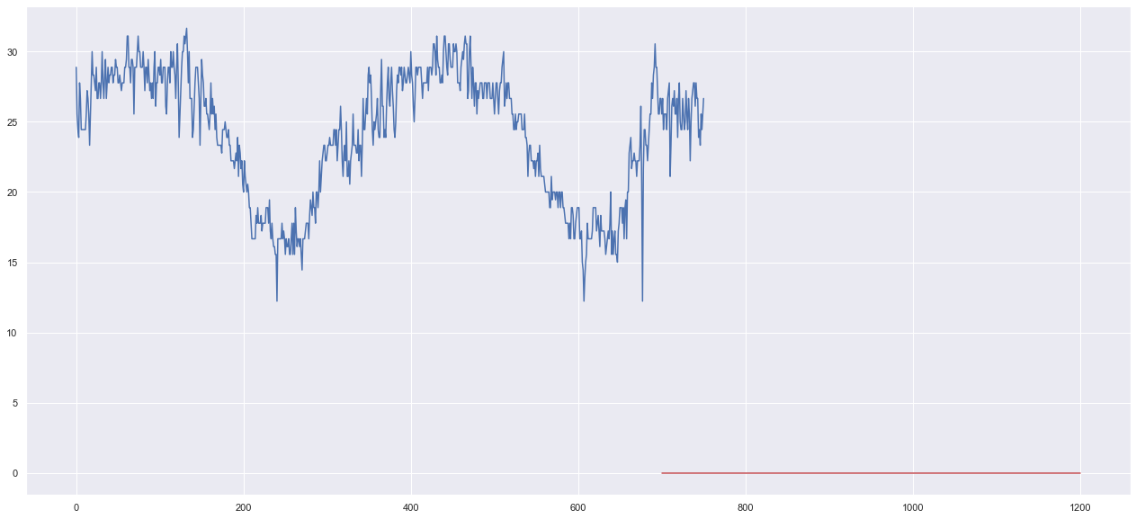
赤色がモデルを元に将来を予測させたものです。
モデルが働いてないですね。
へこたれず次いってみましょう!
2nd try
import statsmodels.api as sm
SARIMA_1_1_1_010 = sm.tsa.SARIMAX(t3_diff, order=(1,1,1), seasonal_order=(0,1,0,300)).fit()
print(SARIMA_1_1_1_010.summary())

residSARIMA = SARIMA_1_1_1_010.resid
fig = plt.figure(figsize=(12,8))
ax1 = fig.add_subplot(211)
fig = sm.graphics.tsa.plot_acf(residSARIMA.values.squeeze(), lags=100, ax=ax1)
ax2 = fig.add_subplot(212)
fig = sm.graphics.tsa.plot_pacf(residSARIMA, lags=100, ax=ax2)

pred = SARIMA_1_1_1_010.predict(700, 1200)

plt.figure(figsize=(22,10))
plt.plot(t3)
plt.plot(pred, "r")
                                  Statespace Model Results
===========================================================================================
Dep. Variable:                            MeanTemp   No. Observations:                  750
Model:             SARIMAX(1, 1, 1)x(0, 1, 0, 300)   Log Likelihood                -969.626
Date:                             Tue, 09 Jul 2019   AIC                           1945.252
Time:                                     18:58:58   BIC                           1957.573
Sample:                                          0   HQIC                          1950.108
                                             - 750
Covariance Type:                               opg
==============================================================================
                 coef    std err          z      P>|z|      [0.025      0.975]
------------------------------------------------------------------------------
ar.L1         -0.1814      0.030     -6.064      0.000      -0.240      -0.123
ma.L1         -0.9997      0.176     -5.688      0.000      -1.344      -0.655
sigma2         4.3343      0.772      5.615      0.000       2.821       5.847
===================================================================================
Ljung-Box (Q):                       87.60   Jarque-Bera (JB):                82.02
Prob(Q):                              0.00   Prob(JB):                         0.00
Heteroskedasticity (H):               1.37   Skew:                            -0.22
Prob(H) (two-sided):                  0.05   Kurtosis:                         5.05
===================================================================================
さっきより少しは良くなりましたかね
でもまだまだです
次
3rd try
周期性が悪いのかと思って360にしてみました。
import statsmodels.api as sm
SARIMA_1_1_1_010 = sm.tsa.SARIMAX(t3_diff, order=(1,1,1), seasonal_order=(0,1,0,360)).fit()
print(SARIMA_1_1_1_010.summary())

residSARIMA = SARIMA_1_1_1_010.resid
fig = plt.figure(figsize=(12,8))
ax1 = fig.add_subplot(211)
fig = sm.graphics.tsa.plot_acf(residSARIMA.values.squeeze(), lags=100, ax=ax1)
ax2 = fig.add_subplot(212)
fig = sm.graphics.tsa.plot_pacf(residSARIMA, lags=100, ax=ax2)

pred = SARIMA_1_1_1_010.predict(700, 1200)

plt.figure(figsize=(22,10))
plt.plot(t3)
plt.plot(pred, "r")
                                  Statespace Model Results
===========================================================================================
Dep. Variable:                            MeanTemp   No. Observations:                  750
Model:             SARIMAX(1, 1, 1)x(0, 1, 0, 360)   Log Likelihood                -821.214
Date:                             Tue, 09 Jul 2019   AIC                           1648.428
Time:                                     20:03:06   BIC                           1660.319
Sample:                                          0   HQIC                          1653.142
                                             - 750
Covariance Type:                               opg
==============================================================================
                 coef    std err          z      P>|z|      [0.025      0.975]
------------------------------------------------------------------------------
ar.L1         -0.2135      0.034     -6.323      0.000      -0.280      -0.147
ma.L1         -0.9999      2.768     -0.361      0.718      -6.426       4.426
sigma2         3.9255     10.872      0.361      0.718     -17.383      25.234
===================================================================================
Ljung-Box (Q):                       71.69   Jarque-Bera (JB):               114.39
Prob(Q):                              0.00   Prob(JB):                         0.00
Heteroskedasticity (H):               1.88   Skew:                            -0.04
Prob(H) (two-sided):                  0.00   Kurtosis:                         5.66
===================================================================================
微妙
次
4th try
import statsmodels.api as sm
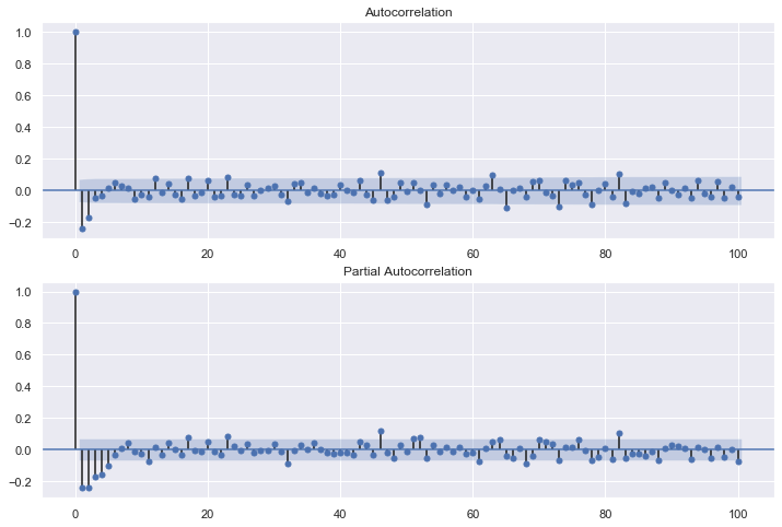
SARIMA_1_0_1_010 = sm.tsa.SARIMAX(t3, order=(1,0,1), seasonal_order=(0,1,0,300)).fit()
print(SARIMA_1_0_1_010.summary())
residSARIMA = SARIMA_1_0_1_010.resid
fig = plt.figure(figsize=(12,8))
ax1 = fig.add_subplot(211)
fig = sm.graphics.tsa.plot_acf(residSARIMA.values.squeeze(), lags=100, ax=ax1)
ax2 = fig.add_subplot(212)
fig = sm.graphics.tsa.plot_pacf(residSARIMA, lags=100, ax=ax2)
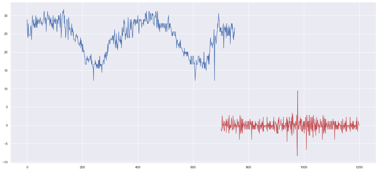
pred = SARIMA_1_0_1_010.predict(700, 1200)
plt.figure(figsize=(22,10))
plt.plot(t3)
plt.plot(pred, "r")
                                  Statespace Model Results
===========================================================================================
Dep. Variable:                            MeanTemp   No. Observations:                  751
Model:             SARIMAX(1, 0, 1)x(0, 1, 0, 300)   Log Likelihood                -955.829
Date:                             Tue, 09 Jul 2019   AIC                           1917.657
Time:                                     20:28:39   BIC                           1929.992
Sample:                                          0   HQIC                          1922.518
                                             - 751
Covariance Type:                               opg
==============================================================================
                 coef    std err          z      P>|z|      [0.025      0.975]
------------------------------------------------------------------------------
ar.L1          0.9701      0.013     75.246      0.000       0.945       0.995
ma.L1         -0.4332      0.037    -11.786      0.000      -0.505      -0.361
sigma2         4.0411      0.183     22.034      0.000       3.682       4.401
===================================================================================
Ljung-Box (Q):                       90.74   Jarque-Bera (JB):               138.85
Prob(Q):                              0.00   Prob(JB):                         0.00
Heteroskedasticity (H):               1.38   Skew:                            -0.53
Prob(H) (two-sided):                  0.05   Kurtosis:                         5.51
===================================================================================
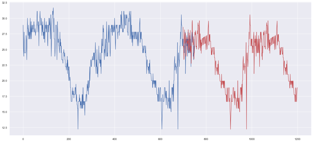
おお!いい感じじゃないですか?
このようなパラメーターの見つけ方をもう少し体系化したいです。
あと、今回うまくいった原因というのもよくわかってません。
AICやBICを確認して小さい物を選ぶといいらしいですが、
モデル間の値をみてみるとそんなに変わらないみたいです。
2nd try AIC = 1945.252
3rd try AIC = 1648.428
4th try AIC = 1917.657 うまくいったやつ
summaryを見てみると、うまくいったモデルはLjung-Box と Jarque-Bera の検定結果の値が大きい傾向にあるようです。
総当たりパラメータ探し
# 総当たりで、AICが最小となるSARIMAの次数を探す
max_p = 3
max_q = 3
max_d = 1
max_sp = 0
max_sq = 0
max_sd = 0

pattern = max_p*(max_q + 1)*(max_d + 1)*(max_sp + 1)*(max_sq + 1)*(max_sd + 1)

modelSelection = pd.DataFrame(index=range(pattern), columns=["model", "aic"])


season = 360

# 自動SARIMA選択
# BICも観ておきたいので改造する
num = 0

for p in range(1, max_p + 1):
    for d in range(0, max_d + 1):
        for q in range(0, max_q + 1):
            for sp in range(0, max_sp + 1):
                for sd in range(0, max_sd + 1):
                    for sq in range(0, max_sq + 1):
                        sarima = sm.tsa.SARIMAX(
                            t3, order=(p,d,q),
                            seasonal_order=(sp,sd,sq,360),
                            enforce_stationarity = False,
                            enforce_invertibility = False
                        ).fit()
                        modelSelection.ix[num]["model"] = "order=(" + str(p) + ","+ str(d) + ","+ str(q) + "), season=("+ str(sp) + ","+ str(sd) + "," + str(sq) + ")"
                        modelSelection.ix[num]["aic"] = sarima.aic
                        modelSelection.ix[num]["bic"] = sarima.bic

                        num = num + 1


# ここはaicを基準にしておこう
# aicが低い順からtop3を出して選べるようにしてもいいかも(ページ下側でやる)
modelSelection[modelSelection.aic == min(modelSelection.aic)]
結果出力
                                aic
order=(1,1,3), season=(0,0,0) 	2525.29
こういう候補を使って試してもうまくはいきませんでした。
なんでや。
総当たり法もう一つ
AIC=[]
BIC=[]
pr_li=[]

p_num = 4
d_num = 4
q_num = 4
trial_num = p_num * d_num * q_num
use_columns = ["p", "d", "q"]
step_cnt = 0
train_data = t3

info_df = pd.DataFrame(index=range(trial_num-2), columns=use_columns)

for p in range(p_num):
    for d in range(d_num):
        for q in range(q_num):
            if p == 0 and q == 0:
                continue
            model = sm.tsa.statespace.SARIMAX(train_data, order=(p, d, q), enforce_invertibility=False, trend='t')
            param_list = [p, d, q]
            for name, val in zip(use_columns[:-1], param_list):
                info_df.iloc[step_cnt][name] = val
            try:
                result = model.fit(disp=False)
                AIC.append(result.aic)
                BIC.append(result.bic)
                pr_li.append(param_list)
            except:
                pass
            step_cnt += 1
            print("Finish trial No. {}, Param: {}".format(step_cnt, param_list))

grid_ser = pd.DataFrame({"palam" : pr_li,
              "AIC" : AIC,
              "BIC" : BIC
             })

so=sorted(grid_ser.AIC)[:5]
grid_ser[grid_ser.AIC==so[0]]

# 結果が1,1,2と出てきたので適応する

model112 =  sm.tsa.statespace.SARIMAX(train_data, order=(1, 1, 2), trend='c')
result112 = model112.fit(disp=False)
print(result112.summary())
参考にしたサイト
季節調整済みARIMAモデルで電力使用状況を推定してみる
http://jbclub.xii.jp/?p=695
PythonでのARIMAモデルを使った時系列データの予測の基礎[後編]
https://blog.brains-tech.co.jp/entry/arima-tutorial-2
Pythonによる時系列分析の基礎
https://logics-of-blue.com/wp-content/uploads/2017/05/python-time-series-analysis-notebook.html#%E6%99%82%E7%B3%BB%E5%88%97%E3%83%87%E3%83%BC%E3%82%BF%E3%81%AE%E5%8F%96%E3%82%8A%E6%89%B1%E3%81%84
python – この時系列は静止しているかどうか
https://codeday.me/jp/qa/20190415/632239.html
statsmodels.tsa.arima_model.ARIMA
https://www.statsmodels.org/stable/generated/statsmodels.tsa.arima_model.ARIMA.html
statsmodels.tsa.statespace.sarimax.SARIMAXResults
https://www.statsmodels.org/dev/generated/statsmodels.tsa.statespace.sarimax.SARIMAXResults.html
R Time Series Analysis 時系列解析(14) SARIMAモデル
http://nakhirot.hatenablog.com/entry/20130716/1373910979
maxlag should be < nobs always OCCUR in python3, how to fix it? #4465
https://github.com/statsmodels/statsmodels/issues/4465
Summary of rules for identifying ARIMA models
http://people.duke.edu/~rnau/arimrule.htm
時系列分析 with Python
http://ytaishiro.hatenablog.com/entry/2018/01/25/053815
How to Create an ARIMA Model for Time Series Forecasting in Python
https://machinelearningmastery.com/arima-for-time-series-forecasting-with-python/
さくっとトレンド抽出: Pythonのstatsmodelsで時系列分析入門
https://data.gunosy.io/entry/statsmodel_trend
Pythonによる時系列分析の基礎
https://logics-of-blue.com/python-time-series-analysis/
新手法例 時系列分析(ARIMAモデル)の機能とその活用
https://www.i-juse.co.jp/statistics/jirei/sympo/10/arima-model.html
SARIMAで時系列データの分析(PV数の予測)
https://www.kumilog.net/entry/sarima-pv
Bug in ARIMA predict(): ValueError: Must provide freq argument if no data is supplied #3534
https://github.com/statsmodels/statsmodels/issues/3534
https://cran.r-project.org/web/packages/forecast/forecast.pdf#Rfn.Arima.1
Amazon Forecast
https://docs.aws.amazon.com/ja_jp/forecast/latest/dg/aws-forecast-recipe-arima.html#aws-forecast-recipe-arima-hyperparamters
時系列解析_理論編
https://logics-of-blue.com/%E6%99%82%E7%B3%BB%E5%88%97%E8%A7%A3%E6%9E%90_%E7%90%86%E8%AB%96%E7%B7%A8/
【時系列】ARIMA(Python)
http://midsum-datasience.hatenablog.com/entry/2018/07/27/094859
statsmodels.tsa.arima_model.ARIMA.fit
https://www.statsmodels.org/devel/generated/statsmodels.tsa.arima_model.ARIMA.fit.html
機械学習による時系列予測
https://logics-of-blue.com/time-series-forecast-by-machine-learning/
A Gentle Introduction to SARIMA for Time Series Forecasting in Python
https://machinelearningmastery.com/sarima-for-time-series-forecasting-in-python/
このあたりやってみてもおもしろそう
anticipy 0.1.6
https://pypi.org/project/anticipy/

時系列データの予測ライブラリ--PyFlux--
https://qiita.com/GushiSnow/items/437dde3293f6d77bfa58