1, introduction
Maximum Entropy Inverse Reinforcement Learning(Brian D. Ziebart, Andrew Maas, J.Andrew Bagnell, and Anind K. Dey, 2008, https://cdn.aaai.org/AAAI/2008/AAAI08-227.pdf) について解説する。
インターネット上ではいくつか日本語の解説記事が見つかったが論文内容に忠実な解説はあまり見つからなかった。
2, 概要
逆強化学習(Inverse Reinforcement Learning)における論文である。逆強化学習とは各状態に報酬が存在し、エージェント(行動の主体)は一連の行動をして得られた報酬の最終的な合計を最大にしようと行動しているとして、そのエージェントの行動履歴から各状態に紐づいた報酬を求めようという強化学習の逆問題である。この論文では最大エントロピーの原理をもととした確率的アプローチで解く手法を提示している。
論文の後半ではタクシーのデータから運転手の経路嗜好をモデル化し、そのうえで最適経路を予測したり、途中までの経路から目的地を予測することが可能になることを示している。
3, 理論
一つのエージェントの一連の行動記録$\zeta$のi番目の状態を$s_i$、その状態でとった行動を$a_i$とする。
状態$s_i$の特徴を表す素性ベクトルを$\mathbf{f}_{s_i}$とする。
この時、行動記録$\zeta$の素性ベクトル$\mathbf{f}_{\zeta}$を各状態の素性ベクトル$\mathbf{f}_{s_i}$の和であらわす。
\mathbf{f}_{\zeta} = \sum_{s \in \zeta}\mathbf{f}_{s}
これは一見乱暴な設定に思えるが、ここではこのモデルでうまくいくように加法性のある素性関数をとることを考えている。
例えば道路の例であれば道路を枝、交差点をノードとするグラフとみなし、ある交差点に居るという状態において左折などの行動をすることで次の状態に遷移すると考える。このとき交差点の通過料金、左折したか否か、道路種別ごとの走行距離(状態を一つ前と現在の交差点の組で定義すれば特徴量にできる)などには特徴量として加法性がある。逆に交差点の気温などの特徴は加法性がない。加法性のない特徴を扱いたい場合は素性関数を工夫する必要があるだろう。
$$\text{reward}(\zeta) = \sum_{s \in \zeta} (\theta^T \mathbf{f}_{s}) = \theta^T \left( \sum_{s \in \zeta} \mathbf{f}_{s} \right) = \theta^T \mathbf{f}_{\zeta} $$
上記の式のように素性ベクトルに対し$\theta^T$をかけることで各状態あるいは行動記録全体についての報酬が計算できるとする。
ベクトル$\theta$は素性ベクトルのそれぞれの要素に対する、報酬を計算するうえでの重み付けを並べたベクトルとして解釈できる。
次に最終的に報酬を逆算するために報酬はどのようにしてエージェントの行動に結びついているのかをモデル化したい。
具体的には報酬が$\theta$で定義されているときある経路$\zeta_i$の実現確率$P(\zeta_i|\theta)$はどうなっているのかを考える。
論文内ではApprenticeship learning via inverse reinforcement learning. (Abbeel, P., and Ng, A. Y. 2004., https://ai.stanford.edu/~ang/papers/icml04-apprentice.pdf) を引用し
推定された報酬によってモデル化されたエージェントが元の学習元のエージェントと同等のパフォーマンスを発揮するための必要十分条件が、モデルにおける素性ベクトルの期待値が学習元のエージェントの素性ベクトルの期待値と一致することであることを示している。数式においては以下である。$\zeta_i$が一連の行動履歴を表しており、左辺ではすべてのあり得る行動履歴について総和を取っている。
$$\sum_{\zeta_i} P(\zeta_i) \mathbf{f}_{\zeta_i} = \tilde{\mathbf{f}} \quad (1) $$
よって$P(\zeta_i|\theta)$が上記の条件を満たしていればそれでよいのだがこのような分布は無数に考えられる上、明確にモデル化することが難しい。
なので論文内ではここで最大エントロピーの原理を導入している。実際、学習元のエージェント(エキスパートと呼ばれる)のデータ以外のことについて何も知らないものとすると、(1)の条件以外の不確かさが最大であるようにモデルを取るのが妥当であろう。
この「不確かさ」をShannonのエントロピーによって表現すると、
\sum_{\zeta_i} P(\zeta_i) \mathbf{f}_{\zeta_i} = \tilde{\mathbf{f}}~,~~\sum_{\zeta_i}P(\zeta_i) = 1
という条件下でエントロピー
-\sum_{\zeta_i} P(\zeta_i)\log P(\zeta_i)
を最大化する$P(\zeta_i)$を求めるというように問題を定義できる。
ラグランジュの未定乗数法でこれを求めると以下(参考:https://mathlog.info/articles/4062 )
$$Z(\theta) = \sum_{i} e^{\theta^T \mathbf{f}_{\zeta_i}}$$
$$P(\zeta_i|\theta) = \frac{1}{Z(\theta)} e^{\theta^T \mathbf{f}_{\zeta_i}} \quad (2) $$
$Z(\theta)$は統計力学との関連から分配関数と呼ばれる。また$\theta$は未定乗数としての役割を果たしている。eの肩に乗っているのはつまるところ$\text{reward}(\zeta_i)$である。
これまで暗黙に状態と行動の組が定まると次の状態が一意に定まるという前提の上で考えていたが、状態遷移も確率的である場合について考えたい。
このとき(3)のようになる。(2)の式が状態遷移を固定した際に実現し、それらが確率的に重ね合わさられている。
$T$は状態遷移確率分布(各(s_i, a_i)についてどの状態にどの確率で遷移するかの分布であり既知)。
$\mathcal{T}$は確率的な遷移によって生じうる全ての未来のシナリオの集合、$o$はそのうちの一つの具体的なシナリオである。$\mathbf{I}{\zeta \in o}$は$o$という状態遷移に設定されいるとき$\zeta$が実現可能かどうかを判定し、可能であれば1を返し不可能であれば0を返す。
$$P(\zeta|\theta, T) = \sum_{o \in \mathcal{T}} P_T(o) \frac{e^{\theta^T \mathbf{f}{\zeta}}}{Z(\theta, o)} \mathbf{I}{\zeta \in o} \quad (3)$$
実際にこれを計算しようとするとありうる遷移の全組み合わせを計算する必要があるがこれは現実的ではないので$Z(\theta,o)$の代わりに状態遷移確率分布において平均化された分配関数である$Z(\theta,T)$を採用することで以下のように近似する。
P(\zeta|\theta, T) \approx \frac{e^{\theta^T \mathbf{f}_{\zeta}}}{Z(\theta, T)}\prod_{s_{t+1}, a_t, s_t \in \zeta} \mathbf{P_T(s_{t+1}|a_t, s_t)}
このようにしてモデル化ができた。これによりある行動$a$をとる確率も以下のように計算できる。$\zeta : a \in \zeta_{t=0}$は$a$から始まる行動記録$\zeta$を表す。
P(\text{action } a | \theta, T) \propto \sum_{\zeta : a \in \zeta_{t=0}} P(\zeta | \theta, T) \quad (5)
それでは逆に学習元エージェントの行動記録から$\theta$を求める方法を考えよう。$\tilde{\zeta}$は学習元エージェントの一連の行動記録である。学習元エージェントの行動をもっともよく説明する報酬を与える$\theta^*$を求めたい。対数尤度を考えて
$$\theta^* = \arg\max_\theta \sum_{\tilde{\zeta}}\log P(\tilde{\zeta}|\theta, T) $$
総和以下を$L(\theta)$と置くと微分は以下のようになる。
$D_{s_i}$は$\theta$設定下でエージェントが$s_i$を訪れる頻度である。
$$\nabla L(\theta) = \tilde{\mathbf{f}} - \sum_{\zeta} P(\zeta|\theta, T)\mathbf{f}_{\zeta} = \tilde{\mathbf{f}} - \sum_{s_i} D_{s_i} \mathbf{f}_{s_i} \quad (6)$$
証明は決定論的な(2)の場合について簡潔に触れるのみにする。
$$L(\theta) = \theta^T \mathbf{f}_{\tilde{\zeta}} - \log(Z(\theta))$$
$$\nabla \left( \theta^T \mathbf{f}_{\tilde{\zeta}} \right) = \mathbf{f}_{\tilde{\zeta}}$$
$$\nabla \log(Z(\theta)) = \frac{1}{Z(\theta)} \sum_{\zeta} e^{\theta^T \mathbf{f}_\zeta} \mathbf{f}_\zeta = \sum_{\zeta} P(\zeta|\theta) \mathbf{f}_\zeta$$
より(6)が従う。
よって$D_{s_i}$がわかれば$\theta$を勾配法で更新できる。
論文内ではこの期待状態訪問頻度$D_{s_i}$を効率よく求めるアルゴリズムを提示している。

(出典:https://cdn.aaai.org/AAAI/2008/AAAI08-227.pdf)
$Z_{s_i}$を$\theta$設定下で状態$s_i$にいるときに今後得られる報酬の総和の期待値とする。Step1,2で$Z_{s_i}$を求める。
Step1では初期値としてすべて1で$Z_{s_i}$を設定している。
Step2では状態$s_i$において行動$a_{i,j}$ ( jは状態$s_i$においてとれる行動のうち何番目であるかを表している)を行ったときに遷移する可能性のあるすべての状態についてそれぞれの状態($s_k$)において、$s_k$になる確率、指数化された$s_k$で得られる報酬、$Z_{s_k}$を掛け合わせたものを計算し、総和を取ることで、行動$a_{i,j}$をしたときに今後得られる報酬の総和の期待値$Z_{a_{i,j}}$を求めている。
そしてこの$Z_{a_{i,j}}$を$j$について集約することで$Z_{s_i}$を更新している。
Step2内のこの2つの操作を交互に十分(少なくとも学習元データの最大系列長より大きいことが望ましい)繰り返すことで今後得られる報酬の総和を考慮した各状態の状態価値と解釈できる$Z_{s_i}$が求まる。Step2のアルゴリズムは強化学習において価値反復法と呼ばれるものに対応する。
$Z_{s_i}$、$Z_{a_{i,j}}$が求まったことで$\zeta$を具体的にシミュレートせずとも$\zeta$の一部分における行動の選択確率が求められるようになった。
Step3では求まった$Z_{s_i}$、$Z_{a_{i,j}}$から各状態$s_i$において行動$a_{i,j}$を行う確率を計算している。
Step4以降では$\zeta$を求まっている部分的な行動選択確率をもとにシミュレートして$D_{s_i}$を求める
Step4では開始地点となる確率で$D_{s_i}$を初期化している。
Step5ではStep3でも求まった各部分での行動の選択確率と既知の遷移確率分布$T$を用いて時間方向に発展させている。
Step6では時間方向を集約することで状態の訪問頻度$D_{s}$としている。
このようにして$D_{s}$がもとまる。よって全体としては
初期の$\theta$を設定したのち
①アルゴリズムを用いて$\theta$から$D_{s}$を計算
②$D_{s}$で$\nabla L(\theta)$を求める
③勾配法で$\theta$を更新
というステップを繰り返すことで$\theta$を求めることができる。
4, Driver Route Modeling
論文の後半ではタクシーのデータを用いて実証実験を行っている。実際に高速道路を好むなどのうまく学習元エージェントの嗜好をモデリングできただけでなく、各径路の総報酬から良い経路を提案したりすることが可能になったことが示されている。
5,実験
簡単な状況設定で実験を行った。
7×7のグリッド上で左上から右下の正の報酬の得られるゴールに向かうが途中に泥マスがあり泥マスを踏むと負の報酬を得るようにした。素性ベクトルは二次元でそれぞれ泥マスかどうかとゴールかどうかを表す。あらかじめ設定した$\theta$は[ 5. -25.]であり、泥マスを踏むとゴールの5倍損をすると解釈できる。
学習前は以下の画像のようであった。左側の図を見ると泥で損をすることなどは当然わかっていない。また右側の図において青い線がエキスパートのデータの動きだが各状態から最終的な報酬が高くなるような方向を示す矢印はまだ学習されておらずバラバラな方向を向いている。

一方学習後のものについて報酬マップを見るとちゃんと泥で損をすることやゴールの価値がわかっている。また矢印をたどれば泥を一度も踏まずにゴールできる経路になっていることがわかるだろう。
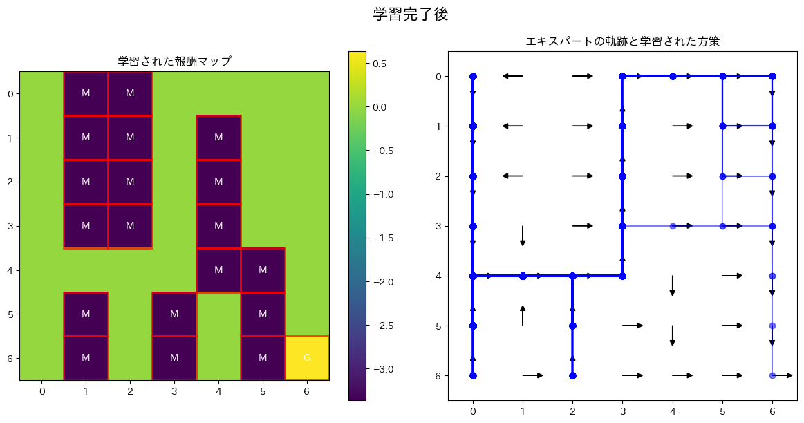
最終的に得られた$\theta$は[ 0.63384785 -3.36456377]であり、価値の割合としては泥マスがゴールの5倍損するということがちゃんととらえられているようであった。
6,コード
実行環境はGoogle Colab
! pip install japanize-matplotlib
import numpy as np
import matplotlib.pyplot as plt
import matplotlib.patches as patches
from matplotlib.colors import ListedColormap
import japanize_matplotlib

class GridWorld:
    def __init__(self, size=5, feature_spec=None):
        self.size = size
        self.num_states = size * size
        self.num_actions = 4  # 0:上, 1:右, 2:下, 3:左

        self.feature_map = {name: i for i, name in enumerate(feature_spec.keys())}
        self.num_features = len(self.feature_map)

        self.features = np.zeros((self.size, self.size, self.num_features))
        for name, positions in feature_spec.items():
            idx = self.feature_map[name]
            for x, y in positions:
                self.features[x, y, idx] = 1

        self.features_flat = self.features.reshape((self.num_states, self.num_features))

        self.transition_prob = self._create_transition_prob()

    def _create_transition_prob(self):
        T = np.zeros((self.num_states, self.num_actions, self.num_states))
        for s in range(self.num_states):
            x, y = self.to_pos(s)

            # 0: 上 1: 右 2: 下 3: 左
            nx, ny = max(0, x - 1), y
            T[s, 0, self.to_state(nx, ny)] = 1.0

            nx, ny = x, min(self.size - 1, y + 1)
            T[s, 1, self.to_state(nx, ny)] = 1.0

            nx, ny = min(self.size - 1, x + 1), y
            T[s, 2, self.to_state(nx, ny)] = 1.0

            nx, ny = x, max(0, y - 1)
            T[s, 3, self.to_state(nx, ny)] = 1.0
        return T

    def to_state(self, x, y):
        return x * self.size + y

    def to_pos(self, s):
        return s // self.size, s % self.size

    def get_rewards(self, theta):
        return self.features_flat @ theta

def compute_state_visitation_freq(grid, theta, trajectories):
    N = max(len(traj) for traj in trajectories)
    rewards = grid.get_rewards(theta)

    # --- ステップ1,2: Backward Pass---
    Z_s = np.zeros((N + 1, grid.num_states))
    Z_s[0, :] = 1.0

    for t in range(1, N + 1):
        Z_a = np.zeros((grid.num_states, grid.num_actions))
        for s_prime in range(grid.num_states):
            s_a_pairs = np.where(grid.transition_prob[:, :, s_prime] > 0)
            for s, a in zip(*s_a_pairs):
                 Z_a[s, a] += np.exp(rewards[s_prime]) * Z_s[t - 1, s_prime]
        Z_s[t, :] = np.sum(Z_a, axis=1)

    # --- ステップ3: 局所的な行動確率の計算 ---
    policy = np.zeros((grid.num_states, grid.num_actions))
    Z_s_N_expanded = np.expand_dims(Z_s[N, :], axis=1)
    Z_a_N = np.zeros((grid.num_states, grid.num_actions))
    for s_prime in range(grid.num_states):
        s_a_pairs = np.where(grid.transition_prob[:, :, s_prime] > 0)
        for s, a in zip(*s_a_pairs):
            Z_a_N[s, a] += np.exp(rewards[s_prime]) * Z_s[N - 1, s_prime] if N > 0 else np.exp(rewards[s_prime])
    # ゼロ除算避
    non_zero_z = Z_s[N, :] != 0
    policy[non_zero_z] = Z_a_N[non_zero_z] / Z_s[N, non_zero_z][:, np.newaxis]


    # --- ステップ4,5: Forward Pass ---
    D = np.zeros((N + 1, grid.num_states))
    start_states = [traj[0] for traj in trajectories]
    unique_starts, counts = np.unique(start_states, return_counts=True)
    D[0, unique_starts] = counts / len(trajectories)

    for t in range(N):
        for s in range(grid.num_states):
            if D[t, s] > 0:
                for a in range(grid.num_actions):
                    s_prime = np.argmax(grid.transition_prob[s, a, :])
                    D[t + 1, s_prime] += D[t, s] * policy[s, a]

    # --- ステップ6: 合計 ---
    state_visitation_freq = np.sum(D, axis=0)
    return state_visitation_freq

def max_ent_irl(grid, trajectories, epochs=20, learning_rate=0.01):
    feature_expectations_expert = np.zeros(grid.num_features)
    for traj in trajectories:
        for state in traj:
            feature_expectations_expert += grid.features_flat[state, :]
    feature_expectations_expert /= len(trajectories)
    theta = np.random.rand(grid.num_features)
    print(f"学習元エージェントの素性ベクトルの期待値: {feature_expectations_expert}")

    for epoch in range(epochs):
        state_visitation_freq = compute_state_visitation_freq(grid, theta, trajectories)
        feature_expectations_model = grid.features_flat.T @ state_visitation_freq
        gradient = feature_expectations_expert - feature_expectations_model
        theta += learning_rate * gradient
    return theta

def generate_expert_trajectories(grid, true_theta, num_trajectories=30, start_state=0, beta=0.5):
    #学習元エージェントを動かすための方策を作成(設定されたtrue_thetaを基に計算された報酬に基づいて価値反復法)
    rewards = grid.get_rewards(true_theta)
    V = np.zeros(grid.num_states)
    for _ in range(100):
        Q = np.zeros((grid.num_states, grid.num_actions))
        for s in range(grid.num_states):
            for a in range(grid.num_actions):
                s_prime = np.argmax(grid.transition_prob[s, a, :])
                Q[s, a] = rewards[s] + 0.9 * V[s_prime] # 割引率0.9
        V = np.max(Q, axis=1)
    Q_stable = Q - np.max(Q, axis=1, keepdims=True)
    exp_q = np.exp(beta * Q_stable)
    stochastic_policy = exp_q / np.sum(exp_q, axis=1, keepdims=True)

    trajectories = []
    for _ in range(num_trajectories):
        traj = []
        state = start_state
        for _ in range(grid.size * 3):
            traj.append(state)
            if grid.to_pos(state) == grid.to_pos(grid.num_states - 1):
                break
            action = np.random.choice(grid.num_actions, p=stochastic_policy[state])
            state = np.argmax(grid.transition_prob[state, action, :])
        trajectories.append(traj)

    return trajectories

def visualize_results(grid, theta, trajectories, title):
    rewards = grid.get_rewards(theta).reshape((grid.size, grid.size))

    fig, ax = plt.subplots(1, 2, figsize=(12, 6))
    fig.suptitle(title, fontsize=16)
    ax[0].set_title("学習された報酬マップ")
    cmap = plt.get_cmap('viridis')
    im = ax[0].imshow(rewards, cmap=cmap)
    fig.colorbar(im, ax=ax[0])
    for name, idx in grid.feature_map.items():
        positions = np.argwhere(grid.features[:, :, idx] == 1)
        for pos in positions:
            rect = patches.Rectangle((pos[1]-0.5, pos[0]-0.5), 1, 1, linewidth=2, edgecolor='red', facecolor='none', alpha=0.7)
            ax[0].add_patch(rect)
            ax[0].text(pos[1], pos[0], name[0].upper(), ha='center', va='center', color='white', weight='bold')
    ax[0].set_xticks(np.arange(grid.size))
    ax[0].set_yticks(np.arange(grid.size))
    ax[1].set_title("エキスパートの軌跡と学習された方策")
    ax[1].imshow(np.zeros_like(rewards), cmap=ListedColormap(['white']))
    for traj in trajectories:
        pos_traj = np.array([grid.to_pos(s) for s in traj])
        ax[1].plot(pos_traj[:, 1], pos_traj[:, 0], marker='o', linestyle='-', alpha=0.3, color='blue')
    V = np.zeros(grid.num_states)
    for _ in range(100):
        Q = np.zeros((grid.num_states, grid.num_actions))
        for s in range(grid.num_states):
            for a in range(grid.num_actions):
                s_prime = np.argmax(grid.transition_prob[s, a, :])
                Q[s, a] = rewards.flatten()[s] + 0.9 * V[s_prime]
        V = np.max(Q, axis=1)
    policy = np.argmax(Q, axis=1)

    for s in range(grid.num_states):
        x, y = grid.to_pos(s)
        action = policy[s]
        dx, dy = 0, 0
        if action == 0: dx = -0.3
        elif action == 1: dy = 0.3
        elif action == 2: dx = 0.3
        elif action == 3: dy = -0.3
        ax[1].arrow(y, x, dy, dx, head_width=0.1, head_length=0.1, fc='black', ec='black')

    ax[1].set_xticks(np.arange(grid.size))
    ax[1].set_yticks(np.arange(grid.size))
    ax[1].set_xlim([-0.5, grid.size-0.5])
    ax[1].set_ylim([grid.size-0.5, -0.5])

    plt.tight_layout(rect=[0, 0, 1, 0.96])
    plt.show()


GRID_SIZE = 7
feature_spec = {
    'goal': [(GRID_SIZE - 1, GRID_SIZE - 1)],
    'mud': [(0,1),(1,1),(2,1),(3,1),(0, 2),(1, 2),(1, 4),(2, 2),(2, 4),(3, 2),(3,4),(4,4),(4,5),(5,3),(6,3),(5,5),(6,5),(5,1),(6,1)]
}
grid = GridWorld(size=GRID_SIZE, feature_spec=feature_spec)
#学習元
true_theta = np.array([5.0, -25.0])
expert_trajectories = generate_expert_trajectories(grid, true_theta, num_trajectories=600, start_state=0)

initial_theta = np.random.rand(grid.num_features)
visualize_results(grid, initial_theta, expert_trajectories, "学習開始前 (初期のランダムな報酬)")

learned_theta = max_ent_irl(grid, expert_trajectories, epochs=30, learning_rate=0.2)

# --- 4. 結果の可視化 ---
print("\n--- 結果 ---")
print(f"真のtheta: {true_theta}")
print(f"学習されたtheta: {learned_theta}")
visualize_results(grid, learned_theta, expert_trajectories, "学習完了後")
7,参考文献
Maximum Entropy Inverse Reinforcement Learning(Brian D. Ziebart, Andrew Maas, J.Andrew Bagnell, and Anind K. Dey, 2008, https://cdn.aaai.org/AAAI/2008/AAAI08-227.pdf)
Apprenticeship learning via inverse reinforcement learning. (Abbeel, P., and Ng, A. Y. 2004., https://ai.stanford.edu/~ang/papers/icml04-apprentice.pdf)
Maximum Entropy Inverse Reinforcementの行間埋め(https://mathlog.info/articles/4062)
日本一詳しくMaximumEntropyIRLのソースコードを解説してみる(https://qiita.com/kinziro/items/3dee1523b9c0a7334c9c)