まえがき
最小二乗法の解説
https://qiita.com/NNNiNiNNN/items/4fd5367f9ead6e5905a9
↑の記事を読んだ前提で説明します。
リッジ回帰とは
最小二乗法における、最小化する目的関数は以下のようなものでした。
E(\mathbf{w}) = ||\mathbf{y} - \mathbf{\tilde{X}\mathbf{w}}||^2
リッジ回帰における、最小化したい目的関数は以下のものです。
E(\mathbf{w}) = ||\mathbf{y} - \mathbf{\tilde{X}\mathbf{w}}||^2 + \lambda ||\mathbf{w} || ^2
ここで加わった$\lambda ||\mathbf{w} || ^2$の項を正則化項といいます。
正則化項とは何かというと、おおざっぱに言って関数の複雑さに対するペナルティです。できるだけ誤差は少なく、しかし関数も複雑にしすぎないように。
今回のリッジ回帰では$\lambda ||\mathbf{w} || ^2$を正則化項として計算します。
λはハイパーパラメータと言いまして、事前に決定しておく定数です。これをいい感じに調整できれば理想的な目的の関数を求められます。
では最小二乗法の場合と同様に$\mathbf{w}$で微分して
\Delta E(\mathbf{w})= -2 \mathbf{\tilde{X}}^T \mathbf{y} + 2 \mathbf{\tilde{X}}^T \mathbf{\tilde{X}}\mathbf{w} +2\lambda \mathbf{w}\\
=2[(\mathbf{\tilde{X}}^T \mathbf{\tilde{X}} + \lambda \mathbf{I})\mathbf{w} - \mathbf{\tilde{X}}^T \mathbf{y}]
これが=0で最小値をとるので、wについて整理して
\mathbf{w} = (\mathbf{\tilde{X}}^T \mathbf{\tilde{X}} + \lambda \mathbf{I})^{-1}\mathbf{\tilde{X}}^T \mathbf{y}
標準化しておきましょう。
(\mathbf{\tilde{X}}^T \mathbf{\tilde{X}} + \lambda \mathbf{I})\mathbf{w} = \mathbf{\tilde{X}}^T \mathbf{y} \tag{1}
これでAx = bの形で解けます。
実装してみよう
基本的に前回と同じコードを使います。
まず訓練用データが
import numpy as np

# y = w[0] + w[1]x[1] + w[2]x[2]型。
# w = [1, 2, 3]とする。
X = np.random.random((100, 2)) * 10 # 0から1*10の範囲をとる100*2の行列
y = 1 + 2 * X[:, 0] + 3 * X[:, 1] + np.random.randn(100)
# x0とx1の座標からyを作成。randnで本来の値にノイズを加えている。
さらに以下を付け加えて
import matplotlib.pyplot as plt
from mpl_toolkits.mplot3d import axes3d
from scipy import linalg # linalg.solve(A, b)

lambda_ = 1 # ハイパーパラメータを1とする。

Xtil = np.c_[np.ones(X.shape[0]), X]
c = np.eye(Xtil.shape[1]) # 単位行列を作る
A = np.dot(Xtil.T, Xtil) + lambda_ * c # (1)式を確認しよう
b = np.dot(Xtil.T, y)
w = linalg.solve(A, b) # (1)式をwについて解く。

xmesh, ymesh = np.meshgrid(np.linspace(0, 10, 20),
                            np.linspace(0, 10, 20))
zmesh = (w[0] + w[1] * xmesh.ravel() +
        w[2] * ymesh.ravel()).reshape(xmesh.shape)

fig = plt.figure()
ax = fig.add_subplot(111, projection='3d')
ax.scatter(X[:, 0], X[:, 1], y, color='k')
ax.plot_wireframe(xmesh, ymesh, zmesh, color='r')
plt.show()
それで出力はこんな感じ。
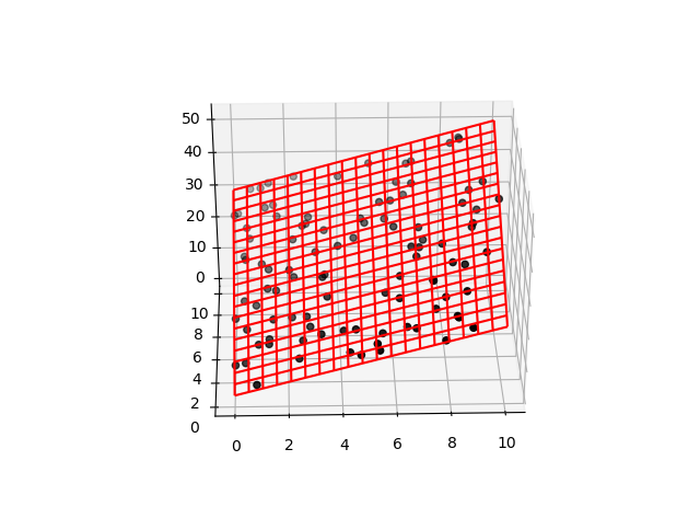
出力できました。
まとめ
リッジ回帰とは回帰分析に正則化項$\lambda ||\mathbf{w} || ^2$を加えたものです。
「関数の複雑さを減らすこと」がどういう意味かは次回、汎化と過学習についてみてみましょう。
『機械学習のエッセンス』という本を参考にしました。この本についてまとめていきます。
前回:最小二乗法
https://qiita.com/NNNiNiNNN/items/4fd5367f9ead6e5905a9
次回:過学習
https://qiita.com/NNNiNiNNN/items/d87990a6eef72a3815a3