画像生成の基本ということで、MNISTのAutoencoderをやってみました。
一年ちょっと前、参考にあるように中間のLatent_dimの大きさが大きければ得られる画像は入力画像のそれとそん色無いというところまでやりました。
今回は、その先へ。。。今日はVAEとちょっとプラスアルファまでやってみようと思います。
どうやらこの先には大きな宝物が埋まっているかもというところにたどり着いたので、あとの楽しみにしてください。
え??そんなの知っていますという方は、以下は読み飛ばしてください。
【参考】
・CapsNetで遊んでみた♬~Autoencoderと比較すると~
やったこと
・MNISTのAutoencoder
・MNISTのVAE
・異常検知について
・MNISTのAutoencoder
ここは、いろいろなコードが考えられ、またMNISTには大仰ですが、以下を採用します。
input_img = Input(shape=(28, 28, 1))  # adapt this if using `channels_first` image data format

x = Conv2D(16, (3, 3), activation='relu', padding='same')(input_img)
x = MaxPooling2D((2, 2), padding='same')(x)
x = Conv2D(8, (3, 3), activation='relu', padding='same')(x)
x = MaxPooling2D((2, 2), padding='same')(x)
x = Conv2D(8, (3, 3), activation='relu', padding='same')(x)
encoded = MaxPooling2D((2, 2), padding='same',name='encoded')(x)
encoder=Model(input_img, encoded)
encoder.summary()

x = Conv2D(8, (3, 3), activation='relu', padding='same')(encoded)
x = UpSampling2D((2, 2))(x)
x = Conv2D(8, (3, 3), activation='relu', padding='same')(x)
x = UpSampling2D((2, 2))(x)
x = Conv2D(16, (3, 3), activation='relu')(x)
x = UpSampling2D((2, 2))(x)
decoded = Conv2D(1, (3, 3), activation='sigmoid', padding='same')(x)

autoencoder = Model(input_img, decoded)
autoencoder.compile(optimizer='adadelta', loss='binary_crossentropy')
autoencoder.summary()
ということで結果は以下のとおりになります。
ちなみに変化が見やすいように1000データで10epoch学習して10000個のTestデータで検証しています。
※今回は精度は問いません
コード全体は以下のとおりです。
VAE/AE_mnist_conv2d.py
・MNISTのVAE
ここは参考の①②を参考にしています。特に参考①③についてはコードをほぼまんま参考にさせていただきました。また、参考②には詳細な説明があって、VAEとはということが理解できます。
【参考】
①KerasでAutoEncoderその2
②Variational Autoencoder徹底解説
③Example of VAE on MNIST dataset using MLP@KerasDocumentation
こうなると、このあたりやる意味あるのかというですが、ウワン的には上記のAEとこのVAEの差分がどうしても知りたいという欲求にかられました。
ということで、おさらいです。
コードの主要な部分は以下のとおりです。
encoderの最初の部分は通常のencoderと同じです。
inputs = Input(shape=input_shape, name='encoder_input')
x = Conv2D(16, (3, 3), activation='relu', padding='same')(inputs)
x = MaxPooling2D((2, 2), padding='same')(x)
x = Conv2D(8, (3, 3), activation='relu', padding='same')(x)
x = MaxPooling2D((2, 2), padding='same')(x)
x = Conv2D(8, (3, 3), activation='relu', padding='same')(x)
x = MaxPooling2D((2, 2), padding='same',name='encoded')(x)
以下で最後のTensorの引数を読込み、shapeに格納します。
そして、latent空間でdecoderの出力を制御したいので、以下のようにFlatten()してから、z_meanとz_log_varという分布の平均値と分散の対数に当たる変数を定義します。
この部分がVAEの主な考え方です。
※つまり、ある分布関数(以下で見るように、z=z_mean + K.exp(0.5 * z_log_var) * epsilonという関数)の変数にlatent空間でとる値を制限して制御する
そして例のLambdaクラスを利用して関数定義することにより、Tensorを引き渡す手法を取っています。
こうして、encoderは入力inputs=input_imgに対して、[z_mean, z_log_var]を出力とするモデルとなります。
shape = K.int_shape(x)
print("shape[1], shape[2], shape[3]",shape[1], shape[2], shape[3])
x = Flatten()(x)
z_mean = Dense(latent_dim, name='z_mean')(x)
z_log_var = Dense(latent_dim, name='z_log_var')(x)
# use reparameterization trick to push the sampling out as input
# note that "output_shape" isn't necessary with the TensorFlow backend
z = Lambda(sampling, output_shape=(latent_dim,), name='z')([z_mean, z_log_var])
# instantiate encoder model
encoder = Model(inputs, [z_mean, z_log_var, z], name='encoder')
encoder.summary()
一方、decoderは入力は上記のLambdaの出力である[z_mean, z_log_var]の二次元の要素を持ったもので、上記のAutoencoderと同様なモデルです。
# build decoder model
# decoder
latent_inputs = Input(shape=(latent_dim,), name='z_sampling')
x = Dense(shape[1] * shape[2] * shape[3], activation='relu')(latent_inputs)
x = Reshape((shape[1], shape[2], shape[3]))(x)
x = Conv2D(8, (3, 3), activation='relu', padding='same')(x)
x = UpSampling2D((2, 2))(x)
x = Conv2D(8, (3, 3), activation='relu', padding='same')(x)
x = UpSampling2D((2, 2))(x)
x = Conv2D(16, (3, 3), activation='relu')(x)
x = UpSampling2D((2, 2))(x)
outputs = Conv2D(1, (3, 3), activation='sigmoid', padding='same')(x)
# instantiate decoder model
decoder = Model(latent_inputs, outputs, name='decoder')
decoder.summary()
# instantiate VAE model
outputs = decoder(encoder(inputs)[2])
vae = Model(inputs, outputs, name='vae_mlp')
一方、Lambdaが定義していた関数samplingは以下のようなもので、これこそがVAEの肝となるものです。
※参考②のReparameterization Trickあたりを見てください
また、参考③のKerasDocumentationにはこの関数に対して以下のコメントがあります
    """Reparameterization trick by sampling for an isotropic unit Gaussian.
    # Arguments
        args (tensor): mean and log of variance of Q(z|X)
    # Returns
        z (tensor): sampled latent vector
    """
ちなみにGauss分布との関係(すなわちパラメータ変換)については以下が参考になります。
【参考】
Reparameterization Trick for Gaussian Distribution
「Assume we have a normal distribution q that is parameterized by θ, specifically $q_θ(x)=N(θ,1)$. We want to solve the below problem
min_θ E_q[x^2]
We want to understand how the reparameterization trick helps in calculating the gradient of this objective $E_q[x^2]$.
One way to calculate $∇_θE_q[x^2]$ is as follows
∇_θE_q[x^2]=∇_θ∫q_θ(x)x^2dx=∫x^2∇_θq_θ(x)\frac{q_θ(x)}{q_θ(x)}dx=∫q_θ(x)∇_θ\log q_θ(x)x^2dx
=E_q[x^2∇_θ\log q_θ(x)]
For our example where qθ(x)=N(θ,1), this method gives
∇_θE_q[x2]=E_q[x^2(x−θ)]
Reparameterization trick is a way to rewrite the expectation so that the distribution with respect to which we take the expectation is independent of parameter θ. To achieve this, we need to make the stochastic element in q independent of θ. Hence, we write x as
x=θ+ϵ,ϵ∼N(0,1)
Then, we can write
E_q[x^2]=E_p[(θ+ϵ)^2]
where p is the distribution of ϵ, i.e., N(0,1). Now we can write the derivative of $E_q[x^2]$ as follows
∇_θE_q[x^2]=∇_θE_p[(θ+ϵ)^2]=E_p[2(θ+ϵ)]
share cite improve this answer」
def sampling(args):
    z_mean, z_log_var = args
    batch = K.shape(z_mean)[0]
    dim = K.int_shape(z_mean)[1]
    # by default, random_normal has mean=0 and std=1.0
    epsilon = K.random_normal(shape=(batch, dim))
    return z_mean + K.exp(0.5 * z_log_var) * epsilon
最後にVAEのloss関数は以下のとおりです。
# Compute VAE loss
reconstruction_loss = binary_crossentropy(K.flatten(inputs), K.flatten(outputs))
reconstruction_loss *= image_size * image_size
kl_loss = 1 + z_log_var - K.square(z_mean) - K.exp(z_log_var)
kl_loss = K.sum(kl_loss, axis=-1)
kl_loss *= -0.5
vae_loss = K.mean(reconstruction_loss + kl_loss)
そして結果は100epochのとき、以下のとおり得られました。

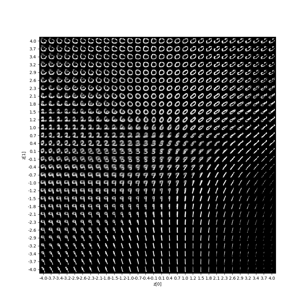
![z_sample_t_No.7_100_50z0=[-0.7,-3]z7=[-0.7,2].gif](https://qiita-user-contents.imgix.net/https%3A%2F%2Fqiita-image-store.s3.ap-northeast-1.amazonaws.com%2F0%2F233744%2F67942ae9-0958-7a7f-0386-2a874211bea4.gif?ixlib=rb-4.0.0&auto=format&gif-q=60&q=75&s=1d4e51ba88ccbe54624b67648b43884c)
コード全体は以下のとおりです。
VAE/keras_vae_conv2d.py
異常検知について
そして参考①で議論されている異常検知、すなわち以下のコードのように学習を7のみに限定して学習すると、そのz空間での様子を見ると以下のようにほぼ全領域で7のような形状になっています。
# 学習に使うデータを限定する
x_train1 = x_train[y_train==7]
x_test1 = x_test[y_test==7]

vae.fit(x_train1,
                epochs=epochs,
                batch_size=batch_size,
                validation_data=(x_test1, None))
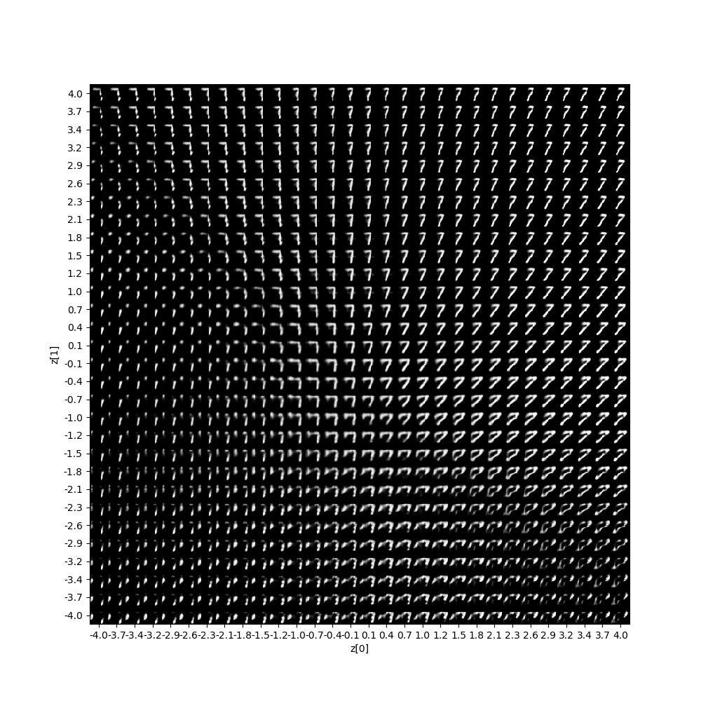
そして異常検知の図は以下のとおりになります。
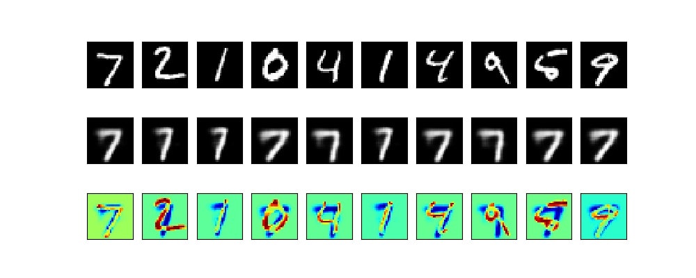
実はここから面白いのですが、この7を学習したモデルでさらに一つずつ文字を学習するとどうなるでしょうか??
DLの記憶って、どうなるか興味がわいたのでやってみましたが、今夜は遅くなったので明日の記事にしたいと思います。
まとめ
・Autoencoderをやってみた
・VAEをやってみた
・異常検知についてやってみた
・DLの記憶ってあるのかどうか明日書きます