 第二夜は、Chainerの基本です。
本書では、わずか7頁の部分ですが、Deeplearningでどのように動くべきか動かすべきかが分かる教育的なコードです。
まず、ChainerのMnistを解説する前にTensorflowとKerasそしてChainerの同様なMnistのコード記載したいと思います。
### 今回説明したいこと
(1)[TensorflowのMnistコード](https://www.tensorflow.org/tutorials/)と実行結果
(2)[KerasのMnistコード](https://github.com/keras-team/keras/blob/master/examples/mnist_cnn.py)と実行結果
(3)[ChainerExampleのMnistコード](https://github.com/chainer/chainer/blob/master/examples/mnist/train_mnist.py)と実行結果
(4)本書のChainerのMnistコードと実行結果
### (1)TensorflowのMnistコードと実行結果
tfとしてtensorflowを呼び出します。
第二夜は、Chainerの基本です。
本書では、わずか7頁の部分ですが、Deeplearningでどのように動くべきか動かすべきかが分かる教育的なコードです。
まず、ChainerのMnistを解説する前にTensorflowとKerasそしてChainerの同様なMnistのコード記載したいと思います。
### 今回説明したいこと
(1)[TensorflowのMnistコード](https://www.tensorflow.org/tutorials/)と実行結果
(2)[KerasのMnistコード](https://github.com/keras-team/keras/blob/master/examples/mnist_cnn.py)と実行結果
(3)[ChainerExampleのMnistコード](https://github.com/chainer/chainer/blob/master/examples/mnist/train_mnist.py)と実行結果
(4)本書のChainerのMnistコードと実行結果
### (1)TensorflowのMnistコードと実行結果
tfとしてtensorflowを呼び出します。
import tensorflow as tf
以下でデータセットmninstを定義して(x_train, y_train),(x_test, y_test)に代入し、さらに規格化します。
mnist = tf.keras.datasets.mnist
(x_train, y_train),(x_test, y_test) = mnist.load_data()
x_train, x_test = x_train / 255.0, x_test / 255.0
以下モデル定義します。
ここでは単純なMLPです。
model = tf.keras.models.Sequential([
  tf.keras.layers.Flatten(),
  tf.keras.layers.Dense(512, activation=tf.nn.relu),
  tf.keras.layers.Dropout(0.2),
  tf.keras.layers.Dense(10, activation=tf.nn.softmax)
])
optimizerとして'adam'を利用し、
lossは'sparse_categorical_crossentropy'
そして、収束のメトリクスは'accuracy'を利用して
モデルをコンパイルします。
model.compile(optimizer='adam',
              loss='sparse_categorical_crossentropy',
              metrics=['accuracy'])
学習の繰り返し数;epoch=10として学習します。
model.fit(x_train, y_train, epochs=10)
以下学習したものを新たなデータセットx_test, y_testを使って検証します。
score = model.evaluate(x_test, y_test, verbose=0)
次に、結果としてlossとaccuracyを表示します。
print('Test loss:', score[0])
print('Test accuracy:', score[1])
以下が上記コードの出力結果です。
上記のコードは行数が少なくある意味分かり易いですが、これ以上の変化はむつかしく、実際どういうことをやっているかは不明です。
60000/60000 [==============================] - 5s 86us/step - loss: 0.2182 - acc: 0.9350
Epoch 2/10
60000/60000 [==============================] - 4s 62us/step - loss: 0.0964 - acc: 0.9711
Epoch 3/10
60000/60000 [==============================] - 4s 62us/step - loss: 0.0686 - acc: 0.9788
Epoch 4/10
60000/60000 [==============================] - 4s 62us/step - loss: 0.0533 - acc: 0.9829
Epoch 5/10
60000/60000 [==============================] - 4s 62us/step - loss: 0.0447 - acc: 0.9855
Epoch 6/10
60000/60000 [==============================] - 4s 62us/step - loss: 0.0354 - acc: 0.9878
Epoch 7/10
60000/60000 [==============================] - 4s 62us/step - loss: 0.0290 - acc: 0.9904
Epoch 8/10
60000/60000 [==============================] - 4s 62us/step - loss: 0.0290 - acc: 0.9906
Epoch 9/10
60000/60000 [==============================] - 4s 62us/step - loss: 0.0241 - acc: 0.9918
Epoch 10/10
60000/60000 [==============================] - 4s 62us/step - loss: 0.0238 - acc: 0.9920
Test loss: 0.07716436276643145
Test accuracy: 0.9824
(2)KerasのMnistコードと実行結果
最初にこのコードのパフォーマンスが記載されています。
そして、必要な関数などをKerasフレームワークからimportしています。
'''Trains a simple convnet on the MNIST dataset.
Gets to 99.25% test accuracy after 12 epochs
(there is still a lot of margin for parameter tuning).
16 seconds per epoch on a GRID K520 GPU.
'''
from __future__ import print_function
import keras
from keras.datasets import mnist
from keras.models import Sequential
from keras.layers import Dense, Dropout, Flatten
from keras.layers import Conv2D, MaxPooling2D
from keras import backend as K
今回学習条件を記載しています。
ここでbatchサイズはまとめて学習する塊のデータ数
mnistではカテゴライズするカテゴリーは0から9の10個です。
あと、epochは上記と同じく学習の繰り返し回数で10回です。
また、mnistの画像サイズは28×28です。
batch_size = 128
num_classes = 10
epochs = 10
# input image dimensions
img_rows, img_cols = 28, 28
Tensorflowと同じように以下でデータを読み込みます。
# the data, split between train and test sets
(x_train, y_train), (x_test, y_test) = mnist.load_data()
以下は画像の、channelと呼ばれる自由度(カラー=3、白黒=1)を前に持ってくるか後に持ってくるかでinput.shapeを成形しています。さらに上記と同じように規格化します。
if K.image_data_format() == 'channels_first':
    x_train = x_train.reshape(x_train.shape[0], 1, img_rows, img_cols)
    x_test = x_test.reshape(x_test.shape[0], 1, img_rows, img_cols)
    input_shape = (1, img_rows, img_cols)
else:
    x_train = x_train.reshape(x_train.shape[0], img_rows, img_cols, 1)
    x_test = x_test.reshape(x_test.shape[0], img_rows, img_cols, 1)
    input_shape = (img_rows, img_cols, 1)

x_train = x_train.astype('float32')
x_test = x_test.astype('float32')
x_train /= 255
x_test /= 255
print('x_train shape:', x_train.shape)
print(x_train.shape[0], 'train samples')
print(x_test.shape[0], 'test samples')
以下で3⇒[0,0,0,1,0,0,0,0,0]みたいにoneHotという形式に変換しています。
# convert class vectors to binary class matrices
y_train = keras.utils.to_categorical(y_train, num_classes)
y_test = keras.utils.to_categorical(y_test, num_classes)
以下がKerasのモデル定義です。
model = Sequential()
model.add(Conv2D(32, kernel_size=(3, 3),
                 activation='relu',
                 input_shape=input_shape))
model.add(Conv2D(64, (3, 3), activation='relu'))
model.add(MaxPooling2D(pool_size=(2, 2)))
model.add(Dropout(0.25))
model.add(Flatten())
model.add(Dense(128, activation='relu'))
model.add(Dropout(0.5))
model.add(Dense(num_classes, activation='softmax'))
そしてTensorflowと同様にlossとoptimizerそしてmetricsを定義して、モデルをコンパイルします。
model.compile(loss=keras.losses.categorical_crossentropy,
              optimizer=keras.optimizers.Adadelta(),
              metrics=['accuracy'])
学習は以下の通りです。検証を毎epochごとに行います。
※ちなみにTensorflowのコードでも以下のようにすると毎epochごとに検証できます。
model.fit(x_train, y_train, epochs=10,validation_data=(x_test, y_test))
model.fit(x_train, y_train,
          batch_size=batch_size,
          epochs=epochs,
          verbose=1,
          validation_data=(x_test, y_test))
最後に学習したmodelで検証してloss等を出力します。
score = model.evaluate(x_test, y_test, verbose=0)
print('Test loss:', score[0])
print('Test accuracy:', score[1])
実行結果は以下のとおりです。
60000/60000 [==============================] - 7s 109us/step - loss: 0.2681 - acc: 0.9175 - val_loss: 0.0603 - val_acc: 0.9801
Epoch 2/10
60000/60000 [==============================] - 4s 71us/step - loss: 0.0910 - acc: 0.9729 - val_loss: 0.0397 - val_acc: 0.9876
Epoch 3/10
60000/60000 [==============================] - 4s 71us/step - loss: 0.0673 - acc: 0.9797 - val_loss: 0.0373 - val_acc: 0.9876
Epoch 4/10
60000/60000 [==============================] - 4s 71us/step - loss: 0.0541 - acc: 0.9841 - val_loss: 0.0350 - val_acc: 0.9883
Epoch 5/10
60000/60000 [==============================] - 4s 71us/step - loss: 0.0473 - acc: 0.9859 - val_loss: 0.0329 - val_acc: 0.9886
Epoch 6/10
60000/60000 [==============================] - 4s 71us/step - loss: 0.0415 - acc: 0.9872 - val_loss: 0.0295 - val_acc: 0.9894
Epoch 7/10
60000/60000 [==============================] - 4s 71us/step - loss: 0.0379 - acc: 0.9887 - val_loss: 0.0254 - val_acc: 0.9917
Epoch 8/10
60000/60000 [==============================] - 4s 71us/step - loss: 0.0340 - acc: 0.9893 - val_loss: 0.0273 - val_acc: 0.9906
Epoch 9/10
60000/60000 [==============================] - 4s 71us/step - loss: 0.0317 - acc: 0.9905 - val_loss: 0.0272 - val_acc: 0.9911
Epoch 10/10
60000/60000 [==============================] - 4s 71us/step - loss: 0.0294 - acc: 0.9913 - val_loss: 0.0262 - val_acc: 0.9909
Test loss: 0.026154597884412215
Test accuracy: 0.9909
(3)Chainer ExampleのMnistコードと実行結果
必要な関数等をchainerフレームワークからimportします。
# !/usr/bin/env python
import argparse
import chainer
import chainer.functions as F
import chainer.links as L
from chainer import training
from chainer.training import extensions
chainerのChainを継承してclass MLPを定義します。
モデルの内容は上記と同じようですが、記述形式が異なっていて、def __init__がコンストラクタ、そして順伝播の処理がdef forwardに記載されています。活性化関数はreluを使っています。
# Network definition
class MLP(chainer.Chain):
    def __init__(self, n_units, n_out):
        super(MLP, self).__init__()
        with self.init_scope():
            # the size of the inputs to each layer will be inferred
            self.l1 = L.Linear(None, n_units)  # n_in -> n_units
            self.l2 = L.Linear(None, n_units)  # n_units -> n_units
            self.l3 = L.Linear(None, n_out)  # n_units -> n_out
    def forward(self, x):
        h1 = F.relu(self.l1(x))
        h2 = F.relu(self.l2(h1))
        return self.l3(h2)
以下上記のモデルを使って、mainで学習します。
下記では外部変数で変更できるbatchsizeなど諸量を定義して読み込んでいます。
def main():
    parser = argparse.ArgumentParser(description='Chainer example: MNIST')
    parser.add_argument('--batchsize', '-b', type=int, default=100,
                        help='Number of images in each mini-batch')
    parser.add_argument('--epoch', '-e', type=int, default=10,
                        help='Number of sweeps over the dataset to train')
    parser.add_argument('--frequency', '-f', type=int, default=-1,
                        help='Frequency of taking a snapshot')
    parser.add_argument('--gpu', '-g', type=int, default=-1,
                        help='GPU ID (negative value indicates CPU)')
    parser.add_argument('--out', '-o', default='result',
                        help='Directory to output the result')
    parser.add_argument('--resume', '-r', default='',
                        help='Resume the training from snapshot')
    parser.add_argument('--unit', '-u', type=int, default=1000,
                        help='Number of units')
    parser.add_argument('--noplot', dest='plot', action='store_false',
                        help='Disable PlotReport extension')
    args = parser.parse_args()

    print('GPU: {}'.format(args.gpu))
    print('# unit: {}'.format(args.unit))
    print('# Minibatch-size: {}'.format(args.batchsize))
    print('# epoch: {}'.format(args.epoch))
    print('')
以下でmodelを定義します。
    # Set up a neural network to train
    # Classifier reports softmax cross entropy loss and accuracy at every
    # iteration, which will be used by the PrintReport extension below.
    model = L.Classifier(MLP(args.unit, 10))
    if args.gpu >= 0:
        # Make a specified GPU current
        chainer.backends.cuda.get_device_from_id(args.gpu).use()
        model.to_gpu()  # Copy the model to the GPU
以下でoptimizerを設定してモデルを作成しています。
    # Setup an optimizer
    optimizer = chainer.optimizers.Adam()
    optimizer.setup(model)
以下でデータセットからbatchsize毎にデータを読み込んで、train_iterとtest_iterに入力します。ここでデータはshuffleしますが、testデータはshuffleしません。
    # Load the MNIST dataset
    train, test = chainer.datasets.get_mnist()
    train_iter = chainer.iterators.SerialIterator(train, args.batchsize)
    test_iter = chainer.iterators.SerialIterator(test, args.batchsize,                                                 repeat=False, shuffle=False)
以下でtrainerを作成します。
    # Set up a trainer
    updater = training.updaters.StandardUpdater(
        train_iter, optimizer, device=args.gpu)
    trainer = training.Trainer(updater, (args.epoch, 'epoch'), out=args.out)
    # Evaluate the model with the test dataset for each epoch
    trainer.extend(extensions.Evaluator(test_iter, model, device=args.gpu))
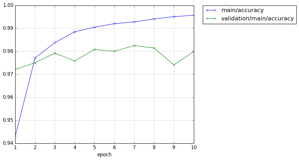
Chainerだと学習途中の表記(グラフ出力など)を以下のように自由に変更できます。
# Dump a computational graph from 'loss' variable at the first iteration
# The "main" refers to the target link of the "main" optimizer.
trainer.extend(extensions.dump_graph('main/loss'))
# Take a snapshot for each specified epoch
frequency = args.epoch if args.frequency == -1 else max(1, args.frequency)
trainer.extend(extensions.snapshot(), trigger=(frequency, 'epoch'))
# Write a log of evaluation statistics for each epoch
trainer.extend(extensions.LogReport())
# Save two plot images to the result dir
if args.plot and extensions.PlotReport.available():
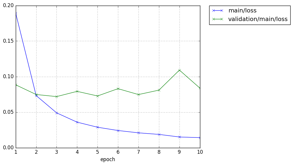
trainer.extend(
extensions.PlotReport(['main/loss', 'validation/main/loss'],
'epoch', file_name='loss.png'))
trainer.extend(
extensions.PlotReport(
['main/accuracy', 'validation/main/accuracy'],
'epoch', file_name='accuracy.png'))
# Print selected entries of the log to stdout
# Here "main" refers to the target link of the "main" optimizer again, and
# "validation" refers to the default name of the Evaluator extension.
# Entries other than 'epoch' are reported by the Classifier link, called by
# either the updater or the evaluator.
trainer.extend(extensions.PrintReport(
['epoch', 'main/loss', 'validation/main/loss',
'main/accuracy', 'validation/main/accuracy', 'elapsed_time']))
# Print a progress bar to stdout
trainer.extend(extensions.ProgressBar())
if args.resume:
# Resume from a snapshot
chainer.serializers.load_npz(args.resume, trainer)
# Run the training
trainer.run()
そして以下のようにグラフがresultに出力されます。
そして、以下は定型のmain()関数呼び出しです。
if __name__ == '__main__':
    main()
一方、標準出力には以下のような出力がされます。
GPU: 0
# unit: 1000
# Minibatch-size: 100
# epoch: 10

epoch       main/loss   validation/main/loss  main/accuracy  validation/main/accuracy  elapsed_time
1           0.189441    0.0884326             0.942917       0.9721                    3.60737
2           0.0733064   0.0747682             0.977099       0.975                     6.29185
3           0.0489878   0.0718525             0.983766       0.9792                    8.97317
4           0.0358914   0.0792011             0.988499       0.9758                    11.6886
5           0.0287545   0.0727362             0.990465       0.9808                    14.3602
6           0.0241362   0.0829734             0.992015       0.98                      17.0939
7           0.0208695   0.0747048             0.992782       0.9825                    19.8217
8           0.0186672   0.0809455             0.994082       0.9814                    22.5557
9           0.0150329   0.109103              0.995082       0.9741                    25.2878
10          0.0141203   0.0837881             0.995665       0.9799                    27.9667
(4)本書のChainerのMnistコードと実行結果
上記の3つのフレームワークにおけるMnistコード解説でほぼわかると思いますが、本書ではさらに初心者にわかりやすいコードそして何をやるべきかに重点を置いて執筆しているのが分かります。
※解説詳細は本書を読んでください
import numpy as np
import chainer
from chainer import Chain
import chainer.functions as F
import chainer.links as L
from chainer import cuda, Variable
from chainer import datasets, iterators, optimizers, serializers
import argparse
ネットワーク定義は通常のclass定義のスタイルを踏襲して、def __call__(self, x):としています。
# ネットワーク定義
class MLP(Chain):
    def __init__(self, n_units):
        super(MLP, self).__init__()
        with self.init_scope():
            self.l1 = L.Linear(None, n_units) # 入力層
            self.l2 = L.Linear(None, n_units) # 中間層
            self.l3 = L.Linear(None, 10)      # 出力層
    def __call__(self, x):
        h1 = F.relu(self.l1(x))
        h2 = F.relu(self.l2(h1))
        return self.l3(h2)
引数はほぼchainerのコードと類似しています。
# 引数の定義
parser = argparse.ArgumentParser(description='example: MNIST')
parser.add_argument('--batchsize', '-b', type=int, default=100,
                    help='Number of images in each mini-batch')
parser.add_argument('--epoch', '-e', type=int, default=10,
                    help='Number of sweeps over the dataset to train')
parser.add_argument('--unit', '-u', default=1000, type=int,
                    help='number of units')
parser.add_argument('--gpu', '-g', type=int, default=-1,
                    help='GPU ID (negative value indicates CPU)')
parser.add_argument('--initmodel', '-m', default='',
                    help='Initialize the model from given file')
parser.add_argument('--resume', '-r', default='',
                    help='Resume the optimization from snapshot')
args = parser.parse_args()

print('GPU: {}'.format(args.gpu))
print('# unit: {}'.format(args.unit))
print('# Minibatch-size: {}'.format(args.batchsize))
print('# epoch: {}'.format(args.epoch))
モデル定義等がシンプルです。
# モデルの作成
model = MLP(args.unit)
# モデルをGPUに転送
if args.gpu >= 0:
    cuda.get_device_from_id(args.gpu).use()
    model.to_gpu()
# 最適化手法の設定
optimizer = optimizers.SGD()
optimizer.setup(model)
モデルの読み込みをここでやっています。
# 保存したモデルを読み込み
if args.initmodel:
    print('Load model from', args.initmodel)
    serializers.load_npz(args.initmodel, model)
# 保存した最適化状態を復元
if args.resume:
    print('Load optimizer state from', args.resume)
    serializers.load_npz(args.resume, optimizer)
データセット読み込みはほぼ同じ
# MNISTデータセットを読み込み
train, test = datasets.get_mnist()

train_iter = iterators.SerialIterator(train, args.batchsize)
test_iter = iterators.SerialIterator(test, args.batchsize, shuffle=False)
以下は
chainer.dataset.concat_examples(batch, device=None, padding=None)
が秀逸な気がする。動きはリンク先のとおりです。データをGPUに送っています。
それ以外はほぼコメントのとおりで、やっていることがわかりやすいと思います。
以下が学習に相当する部分です。tensorflow.kerasのコード言えば
model.fit(x_train, y_train, epochs=10)
に相当する部分の中身でやっていることです。
# 学習ループ
for epoch in range(1, args.epoch + 1):
    # ミニバッチ単位で学習
    sum_loss = 0
    itr = 0
    for i in range(0, len(train), args.batchsize):
        # ミニバッチデータ
        train_batch = train_iter.next()
        x, t = chainer.dataset.concat_examples(train_batch, args.gpu)
        # 順伝播
        y = model(x)
        # 勾配を初期化
        model.cleargrads()
        # 損失計算
        loss = F.softmax_cross_entropy(y, t)
        # 誤差逆伝播
        loss.backward()
        optimizer.update()
        sum_loss += loss.data
        itr += 1
そして、評価すなわちtensorflow.kerasの以下のコードに対応する部分です。
score = model.evaluate(x_test, y_test, verbose=0)
が以下のように書き下しされています。何をやっているかわかります。
    # 評価
    sum_test_loss = 0
    sum_test_accuracy = 0
    test_itr = 0
    for i in range(0, len(test), args.batchsize):
        # ミニバッチデータ
        test_batch = test_iter.next()
        x_test, t_test = chainer.dataset.concat_examples(test_batch, args.gpu)
        # 順伝播
        y_test = model(x_test)
        # 損失計算
        sum_test_loss += F.softmax_cross_entropy(y_test, t_test).data
        # 一致率計算
        sum_test_accuracy += F.accuracy(y_test, t_test).data
        test_itr += 1
    print('epoch={}, train loss={}, test loss={}, accuracy={}'.format(
        optimizer.epoch + 1, sum_loss / itr,
        sum_test_loss / test_itr, sum_test_accuracy / test_itr))
    optimizer.new_epoch()
最後にモデルを保存します。
# モデル保存
print('save the model')
serializers.save_npz('mlp.model', model)
# 最適化状態保存
print('save the optimizer')
serializers.save_npz('mlp.state', optimizer)
結果は以下の通りになりました。結果見るとDouble以上で計算しているみたいです。
GPU: -1
# unit: 1000
# Minibatch-size: 100
# epoch: 10
epoch=1, train loss=1.0623023396233717, test loss=0.48133535012602807, accuracy=0.8835000020265579
epoch=2, train loss=0.4172537006686131, test loss=0.34605228919535874, accuracy=0.9064999985694885
epoch=3, train loss=0.3360347547630469, test loss=0.30162001533433797, accuracy=0.9155000013113022
epoch=4, train loss=0.29861836368838945, test loss=0.2754953534528613, accuracy=0.9230000019073487
epoch=5, train loss=0.2734103119373322, test loss=0.25352123415097594, accuracy=0.9279000014066696
epoch=6, train loss=0.25372244119644166, test loss=0.23997037421911954, accuracy=0.9309000027179718
epoch=7, train loss=0.2374487419674794, test loss=0.22784614588133992, accuracy=0.9350000029802322
epoch=8, train loss=0.22315640721470117, test loss=0.2145309145655483, accuracy=0.9381000036001206
epoch=9, train loss=0.2105092981768151, test loss=0.20345919621177017, accuracy=0.9417000037431716
epoch=10, train loss=0.19940912450353304, test loss=0.19285368533805014, accuracy=0.9449000054597855
save the model
save the optimizer
まとめ
・Tensorflow、Keras、そしてChainerと本書記載のChainerのMNISTのプログラムを比較解説した
・モデルやoptimizerの違いなどもあり、何が優れているという結論をだそうとするものではない
・今回は基本のきであり、将棋AIとしてどういう機能が必要かは今後見ていきたいと思う