【アニメーション入門】定番FuncAnimation関数で遊んでみた♬

これまで、この関係ではいくつか記事を書いてきましたが、今回のものが定番でしょう。
よく見ると、アニメーションのさせ方はいくつかに分類できるということに気が付いたのでそちらのまとめをします。
【参考】
①matplotlib のanimation を保存@はしくれエンジニアもどきのメモ
②matplotlibのanimation.FuncAnimationを用いて柔軟にアニメーション作成
③Animated line plot@matplotlib
④【シミュレーション入門】サイン波のマスゲーム♬

やったこと

・簡単なアニメーション
・updateを使っている
・yeildを使う
・matplotlibの描画１
・FuncAnimation()関数の仕様
・FuncAnimation()関数の仕様を意識して描画する
・リサジュー図形を描く

・簡単なアニメーション

たぶん一番簡単に動かしているコード
※このコード派生が見やすいので、比較のために全コード引用させていただきます
以下のコードでは、位相aを変化させてsin波を計算し、imでプロットし、それを配列imsに格納してanimationしています。
つまり、こういう風にプロットの集合を順次animationできるという例となっています。

簡単なアニメーションのコード

import numpy as np
import matplotlib.pyplot as plt
import matplotlib.animation as animation

fig = plt.figure()
x = np.arange(0, 10, 0.1)
ims = []
for a in range(50):
    y = np.sin(x - a)
    im = plt.plot(x, y, "b")
    ims.append(im)

ani = animation.ArtistAnimation(fig, ims)
ani.save('sample.gif', writer='imagemagick')

・updateを使っている

以下は、参考②のコードです。解説も丁寧にされているので詳細はそちらを見るといいと思います。
簡単に解説すると、上記ではいちいち計算しplotしていたものをupdate関数に入れて、これをFuncAnimation関数から呼び出すことにより描画しています。
考え方として、毎回前回の描画をplt.cla()で消去して描画するというパラパラ漫画の神髄を言っていると思います。

update関数利用の簡単なアニメーションのコード

import matplotlib.animation as anm
import matplotlib.pyplot as plt
import numpy as np

fig = plt.figure(figsize = (10, 6))
x = np.arange(0, 10, 0.1)

def update(i, fig_title, A):
    if i != 0:
        plt.cla()                      # 現在描写されているグラフを消去
        pass
    y = A * np.sin(x - i)
    plt.plot(x, y, "r")
    plt.title(fig_title + 'i=' + str(i))

ani = anm.FuncAnimation(fig, update, fargs = ('Initial Animation! ', 2.0), \
    interval = 100, frames = 132)
ani.save("Sample1.gif", writer = 'imagemagick')

・yeildを使う

以下のコードは、generator関数を利用しています。

generator関数利用の簡単なアニメーションのコード

import numpy as np
import matplotlib.pyplot as plt
from matplotlib.animation import FuncAnimation

fig = plt.figure(figsize=(8, 8))
ax = plt.subplot(111, frameon=True)

x = np.arange(0, 10, 0.1)
y = np.sin(x)
lin, = ax.plot(x,y,'ro')

def gen(n):
    i = 0
    n = n
    while i < n:
        y = np.sin(x-i)
        yield y
        i +=  1
        
def update(num, data_, line):
    y1= next(data_)
    line.set_data(x,y1)

data_ = gen(1000)
N = 100
anim = FuncAnimation(fig, update, N, fargs=(data_, lin), interval=100)
anim.save("Sample2.gif", writer = 'imagemagick')

・matplotlibの描画１

matplotlibのサンプルとして、上記参考③に掲載されているもの。
animate()関数という上記のupdate()関数と同じ役割の関数において、初期化でplotしたlineに対して、line.set_ydataでデータ更新することにより、動画描画している。
※動画を滑らかに連続させるために2*np.piを加筆、
　また、位相の変化の符号が異なるので逆方向に移動している

matplotlibの例の簡単なアニメーションのコード

import numpy as np
import matplotlib.pyplot as plt
import matplotlib.animation as animation

fig, ax = plt.subplots()

x = np.arange(0, 2*np.pi, 0.01)
line, = ax.plot(x, np.sin(x))

def animate(i):
    line.set_ydata(np.sin(x + 2*np.pi*i / 50))  # update the data.
    return line,

ani = animation.FuncAnimation(
    fig, animate, interval=20, blit=True, save_count=50)
ani.save("animated_line_plot.gif")

上記のコードと比較すると、animate()関数にreturn line, が必要なのかと疑問を持ち以下のコードをやってみると、やはり動きました。

matplotlibの簡単なアニメーションのコードII

import numpy as np
import matplotlib.pyplot as plt
import matplotlib.animation as animation

fig, ax = plt.subplots()

x = np.arange(0, 2*np.pi, 0.01)
line, = ax.plot(x, np.sin(x))

def animate(i):
    line.set_ydata(np.sin(x - 2*i*np.pi / 50))  # update the data.
    #return line,

ani = animation.FuncAnimation(
    fig, animate, interval=20) #, blit=True) #, save_count=50)
    
ani.save("animated_line_plot.gif")

・FuncAnimation()関数の仕様

上記の特に最後の描画を理解するために、ここでアニメーション関数の仕様を見ておきましょう。
引数は、以下のようになっています。これらの引数に対して参考⑤で解説がありますので、それを掲載します。
class matplotlib.animation.FuncAnimation(fig, func, frames=None, init_func=None, fargs=None, save_count=None, *, cache_frame_data=True, **kwargs)[source]
【参考】
⑤matplotlib.animation.FuncAnimation

名称	引数	解説
fig	Figure
func	callable	各フレームで呼び出す関数。最初の引数は、フレーム内の次の値になります。追加の位置引数は、fargsパラメーターを介して指定できます。必要な書式は次のとおりです。 def func(frame, *fargs) -> iterable_of_artists \textrm{blit == True}の場合、funcは、変更または作成されたすべてのアーティストの反復可能オブジェクトを返す必要があります。この情報は、図のどの部分を更新する必要があるかを決定するためにブリッティングアルゴリズムによって使用されます.blit == Falseの場合、戻り値は使用されません。その場合は省略できます。
frames	iterable, int, generator function, or None, optional	funcとアニメーションの各フレームを渡すためのデータのソース ・反復可能である場合は、提供された値を使用するだけです。 iterableに長さがある場合、 save_count　kwargをオーバーライドします。 ・整数の場合、range(frames)を渡すのと同じです ・ジェネレーター関数の場合、以下の書式が必要です。 def gen_function() -> obj ・Noneの場合、itertools.countを渡すのと同じです。 これらすべての場合において、フレーム内の値はユーザー提供の関数に渡されるだけなので、どのタイプでもかまいません。
init_func	callable, optional	明確なフレームを描画するために使用される関数。指定しない場合は、フレームシーケンスの最初のアイテムから描画した結果が使用されます。この関数は、最初のフレームの前に1回呼び出されます。必要な書式は次のとおりです。def init_func() -> iterable_of_artistsblit == Trueの場合、init_funcは、再描画されるアーティストの反復可能オブジェクトを返す必要があります。この情報は、図のどの部分を更新する必要があるかを決定するためにブリッティングアルゴリズムによって使用されます。 blit == Falseの場合、戻り値は使用されません。その場合は省略できます。
fargs	tuple or None, optional	funcへの各呼び出しに渡す追加の引数。
save_count	int, default: 100	フレームからキャッシュへの値の数のフォールバック。これは、フレーム数をフレームから推測できない場合、つまり、長さのないイテレータまたはジェネレータである場合にのみ使用されます。
interval	int, default: 200	ミリ秒単位のフレーム間の遅延。
repeat_delay	int, default: 0	繰り返しがTrueの場合、連続するアニメーションの実行間のミリ秒単位の遅延。
repeat	bool, default: True	フレームのシーケンスが完了したときにアニメーションが繰り返されるかどうか。
blit	bool, default: False	描画を最適化するためにブリッティングが使用されているかどうか。注：ブリッティングを使用する場合、アニメーション化されたアーティストはzorderに従って描画されます。ただし、zorderに関係なく、以前のアーティストの上に描画されます。
cache_frame_data	bool, default: True	フレームデータをキャッシュするかどうか。フレームに大きなオブジェクトが含まれている場合は、キャッシュを無効にすると役立つ場合があります。
・zorderって何よというのは、以下の参考⑥⑦から描画面をx-yとすると、z軸の表示順（前面-背面；数字0-）を決める数字だそうです。
以下は、参考⑦からの引用です。(番号の大きいほど、前面)
The default value depends on the type of the Artist:

Artist	Z-order
Images (AxesImage, FigureImage, BboxImage)	0
Patch, PatchCollection	1
Line2D, LineCollection (including minor ticks, grid lines)	2
Major ticks	2.01
Text (including axes labels and titles)	3
Legend	5

【参考】
⑥matplotlibの表示順に関する設定
⑦Zorder Demo@matplotlib

・FuncAnimation()関数の仕様を意識して描画する

上記と同じようなサイン波を仕様を意識して描いて見ます。
【参考】
⑧【Matplotlib】FuncAnimationクラスを使用してグラフ内にアニメーションを描画する

blit=Falseの場合

上の参考⑧のコードをサイン波出力に変更しています。

FuncAnimation関数の仕様を意識したアニメーションのコード

import numpy as np
import matplotlib.pyplot as plt
import matplotlib.animation as animation

fig = plt.figure(figsize=(8, 6))
ax = fig.add_subplot(1, 1, 1)
line,= ax.plot([], [])
print("start")

def gen_function():
    """
    ジェネレーター関数
    """
    x = []
    y = []
    for i in range(100):
        x0 = np.float(i*np.pi/50.)
        y0 = np.sin(x0) # ~~xの要素を逆順にする~~
        x.append(x0)
        y.append(y0)
    for _x, _y in zip(x, y):
        yield [_x, _y] # 要素要素を戻り値として返す

def init():
    x = np.arange(0, 10, 0.1)
    y = np.sin(x)
    ax.set_xlim(0, 2*np.pi)
    ax.set_ylim(-1.1,1.1)
    line, = ax.plot(x, y, 'black')
    print("called?")

def plot_func(frame):
    """
    frame[0]: _xの要素
    frame[1]: _yの要素
    """
    print(frame[0], frame[1])
    ax.plot(frame[0],frame[1], 'ro')
    plt.pause(0.1) #パラパラ漫画となっている

ani = animation.FuncAnimation( #blit = Falseの場合
    fig=fig,
    func=plot_func,
    frames=gen_function, # ジェネレーター関数を設定
    init_func=init,
    repeat=True,
    save_count = 100,
)

ani.save("animated_line_plot_savecount150.gif")
plt.show()

blit=Trueの場合;zorderを意識して描く

zorderを使いこなすためにより仕様を意識して描画してみました。

zorderを利用の簡単なアニメーションのコード

import matplotlib.pyplot as plt
from matplotlib.animation import FuncAnimation
import numpy as np

x_data = []
y_data = []

fig, ax = plt.subplots()
line,= ax.plot([], [], 'ro', zorder = 1) #zorder=1背面
line_, = ax.plot([], [],zorder = 2, linewidth = 3) #zoder=2 前面

def gen_function():
    x = []
    y = []
    for i in range(100):
        x0 = np.float(i*np.pi/50.)
        y0 = np.sin(x0)
        x.append(x0)
        y.append(y0)
    for _x, _y in zip(x, y):
        yield [_x, _y] # 要素要素を戻り値として返す

def init():
    """
    初期化関数
    """
    ax.set_xlim(0, 2*np.pi) # x軸固定
    ax.set_ylim(-1.1, 1.1) # y軸固定
    del (x_data[:], y_data[:]) # データを削除
    return line, #line_, # 初期化されたプロットを返す

def plot_func(frame):
    """
    frameにはジェネレーター関数の要素が代入される
    frame: [_x, _y]
    """
    x_data.append(frame[0]) #x_data =frame[0]
    y_data.append(frame[1]) #y_data = frame[1]
    line.set_data(x_data, y_data) # 繰り返しグラフを描画
    line_.set_data(x_data, y_data) # 繰り返しグラフを描画
    return line, #line_, # 更新されたプロットを返す

anim = FuncAnimation(
    fig=fig,
    func=plot_func,
    frames=gen_function,
    init_func=init,
    interval=100,
    repeat=True,
    blit = True,
    save_count = 100,
)
anim.save("anime_generator_savecount100_zorder_12_.gif")
plt.show()

ここで、line, はプロット描画、line_, は線描画です。
また、zorder=1は、zorder =2 より背面側に描画されます。

そして、この場合、以下のline, とline_の返却のお作法が少なくとも４種類はあります。
return line, #line_, # 初期化されたプロットを返す
return line, #line_, # 更新されたプロットを返す
やってみると、以下の通りとなります。
・何も返さない⇒blit = Trueとしているのでエラーになります。
・line, line_, 両方返す　line, line_, がzorder = 1, 2の場合

・line, line_, 両方返す　line, line_, がzorder = 2, 1の場合
プロットが線に隠れなくなって一安心

・line, のみ 両方返す　line, line_, がzorder = 2, 1の場合
このコードだと、この場合も上のものと全く同じanim.saveの画像が得られました。
実際の画面上でのplt.show()では上のblit=Falseと同じような描画が表れますが、保存されたgifは「・line, line_, 両方返す　line, line_, がzorder = 2, 1の場合」と同じです。
さてということで、以下のように明示的にline_を外だしして、animationから外して描くこととしました。コードを見ると分かると思いますが、最初のline_の定義の所でまず描画します。そのあとは上記のコードと同一ですが、#line_.set_data(x_data, y_data)として、データの置き換えを実施しないこととしています。これを残しておくと、やはり上記と同じように描画上はサイン波の全体像は残りますが、保存されたものは「・line, line_, 両方返す　line, line_, がzorder = 2, 1の場合」と同じです。

zorder利用の簡単なアニメーションのコードII

import matplotlib.pyplot as plt
from matplotlib.animation import FuncAnimation
import numpy as np

x_data = []
y_data = []

fig, ax = plt.subplots()
line,= ax.plot([], [], 'ro', zorder = 1)

x = np.arange(0, 10, 0.1)
y = np.sin(x)
line_, = ax.plot(x, y,zorder = 2, linewidth = 3)

def gen_function():
    x = []
    y = []
    for i in range(100):
        x0 = np.float(i*np.pi/50.)
        y0 = np.sin(x0) #
        x.append(x0)
        y.append(y0)
    for _x, _y in zip(x, y):
        yield [_x, _y] # 要素要素を戻り値として返す

def init():
    """
    初期化関数
    """
    ax.set_xlim(0, 2*np.pi) # x軸固定
    ax.set_ylim(-1.1, 1.1) # y軸固定
    del (x_data[:], y_data[:]) # データを削除
    return line, #line_, # 初期化されたプロットを返す

def plot_func(frame):
    """
    frameにはジェネレーター関数の要素が代入される
    frame: [_x, _y]
    """
    x_data.append(frame[0]) #x_data =frame[0]
    y_data.append(frame[1]) #y_data = frame[1]
    line.set_data(x_data, y_data) # 繰り返しグラフを描画
    #line_.set_data(x_data, y_data) # 繰り返しグラフを描画
    return line, #line_, # 更新されたプロットを返す

anim = FuncAnimation(
    fig=fig,
    func=plot_func,
    frames=gen_function,
    init_func=init,
    interval=100,
    repeat=True,
    blit = True,
    save_count = 150,
)
anim.save("new_anime_generator_savecount100_zorder_12_both_.gif")

ということで、元々やりたかったことが以下のように出来ました。
ちゃんと、定義通りに描画順序を正しく反映して、しかも元々やりたかったblit=Falseの場合と同じ描画が得られました。
・zorderを1，2とした場合

・zorderを2，1とした場合

・リサジュー図形を描く

FuncAnimationの仕様を意識して最初のサイン波の位相を動かす

リサジュー図形を描くためにx方向、ｙ方向へ進行する波形を描画する

まずは、リサジュー図形のための、x方向、ｙ方向へ進行する波形を表します。
上のままのコードをちょっと変更しました。

リサジュー図形のためのサイン波の簡単なアニメーションのコード

import matplotlib.pyplot as plt
from matplotlib.animation import FuncAnimation
import numpy as np

x_data = []
y_data = []

fig, ax = plt.subplots()
line,= ax.plot([], [], 'ro', zorder = 2)
x = np.arange(-np.pi, np.pi, 0.1)
y = np.pi*np.sin(x)
line_, = ax.plot(x, y,zorder = 1, linewidth = 3)

def gen_function():
    x0 = np.arange(-np.pi, np.pi, 0.1)
    y0 = np.pi*np.sin(x)
    for i in range(100):
        y0 = np.pi*np.sin(x-i*np.pi/50) #毎回位相を変えて一周期分計算してyoに代入
        yield [x0, y0] # 要素要素を戻り値として返す
        
def init():
    """
    初期化関数
    """
    ax.set_xlim(-np.pi-0.1, np.pi+0.1) # x軸固定
    ax.set_ylim(-np.pi-0.1, np.pi+0.1) # y軸固定
    del (x_data[:], y_data[:]) # データを削除
    return line, line_, # 初期化されたプロットを返す

def plot_func(frame):
    """
    frameにはジェネレーター関数の要素が代入される
    frame: [_x, _y]
    """
    x_data =frame[0] #frame[0]で1周期分のデータ
    y_data =frame[1] 
    line.set_data(x_data, y_data) # 繰り返しグラフを描画
    line_.set_data(y_data, x_data) # y方向への進行波
    return line, line_, # 更新されたプロットを返す

anim = FuncAnimation(
    fig=fig,
    func=plot_func,
    frames=gen_function,
    init_func=init,
    interval=100,
    repeat=True,
    blit = True,
    save_count = 150,
)
anim.save("anime_generator_savecount100_zorder_21_ressajous_.gif")
plt.show()

描画結果は、以下のとおりになりました。

リサジュー図形を描く

３つの図形を同時に描画します。見やすいようにx-, y-軸方向への進行波を線描画、ressajyousをプロットで描画します。

コードは以下のとおりです。

リサジュー図形のアニメーションのコード

import matplotlib.pyplot as plt
from matplotlib.animation import FuncAnimation
import numpy as np

x_data = []
y_data = []
y1_data = []

fig, ax = plt.subplots()
line,= ax.plot([], [], zorder = 2, linewidth = 3)
x = np.arange(-np.pi, np.pi, 0.1)
y = np.pi*np.sin(x)
y1 = np.pi*np.sin(2*x)
line_, = ax.plot(x, y1,zorder = 1, linewidth = 3)
line_1, = ax.plot(y, y1,'ro', zorder = 3)

def gen_function():
    x0 = np.arange(-np.pi, np.pi, 0.1)
    for i in range(100):
        y0 = np.pi*np.sin(x-i*np.pi/50)
        y1 = np.pi*np.sin(2*(x-i*np.pi/50)+i*np.pi/50) #位相をずらす
        yield [x0, y0, y1] # 3要素を戻り値として返す
        
def init():
    """
    初期化関数
    """
    ax.set_xlim(-np.pi-0.1, np.pi+0.1) # x軸固定
    ax.set_ylim(-np.pi-0.1, np.pi+0.1) # y軸固定
    del (x_data[:], y_data[:], y1_data[:]) # データを削除
    return line, line_, line_1, # 初期化されたプロットを返す

def plot_func(frame):
    """
    frameにはジェネレーター関数の要素が代入される
    frame: [_x, _y]
    """
    x_data =frame[0]
    y_data =frame[1]
    y1_data =frame[2]
    line.set_data(x_data, y_data) # 繰り返しグラフを描画
    line_.set_data(y1_data, x_data) 
    line_1.set_data(y_data, y1_data)
    return line, line_, line_1, # 更新されたプロットを返す

anim = FuncAnimation(
    fig=fig,
    func=plot_func,
    frames=gen_function,
    init_func=init,
    interval=100,
    repeat=True,
    blit = True,
    save_count = 150,
)
anim.save("anime_generator_savecount100_zorder_21_ressajous_b.gif")
plt.pause(10)

リサジュー図形を描くII

今度は、リサジュー図形の説明の意味でx-, y- 方向へのサイン波上のプロットの（振幅、振幅）図つまりリサジューを描きます。

リサジュー図形のアニメーションのコードII

import matplotlib.pyplot as plt
from matplotlib.animation import FuncAnimation
import numpy as np

x_data = []
y_data = []
y1_data = []


fig, ax = plt.subplots()
line,= ax.plot([], [], zorder = 2, linewidth = 3)
x = np.arange(-np.pi, np.pi, 0.01)
y = np.pi*np.sin(x)
y1 = np.pi*np.sin(2*x)
line_, = ax.plot(x, y1,zorder = 1, linewidth = 1)
line1_, = ax.plot(y, x,zorder = 1, linewidth = 1)
line_1, = ax.plot([], [],'bo',markersize=12, zorder = 3.1)
line_11, = ax.plot(y, y1, zorder = 3, linewidth = 2)
line2,= ax.plot([], [], 'ro', zorder = 2)
line_2, = ax.plot([], [], 'go',zorder = 1 )


def gen_function():
    x_ = []
    y_ = []
    y1_ = []
    for j in range(400):
        x0_ = np.float(j*np.pi/100.-np.pi)
        y0_ = np.pi*np.sin(2*x0_)
        y10_ = np.pi*np.sin(x0_)
        x_.append(x0_)
        y_.append(y0_)
        y1_.append(y10_)
    for _x, _y, _y1 in zip(x_, y_, y1_):
        yield [_x, _y, _y1] # 要素要素を戻り値として返す
        
def init():
    """
    初期化関数
    """
    ax.set_xlim(-np.pi-0.1, np.pi+0.1) # x軸固定
    ax.set_ylim(-np.pi-0.1, np.pi+0.1) # y軸固定
    del (x_data[:], y_data[:], y1_data[:] ) # データを削除
    return line2, line_2, line_1,  # 初期化されたプロットを返す

def plot_func(frame):
    """
    frameにはジェネレーター関数の要素が代入される
    frame: [_x, _y]
    """
    x_data =frame[0]
    y_data =frame[1]
    y1_data = frame[2]
    line2.set_data(x_data, y_data) # 繰り返しグラフを描画
    line_2.set_data(y1_data, x_data)
    line_1.set_data(y1_data, y_data)
    return line2, line_2, line_1,  # 更新されたプロットを返す

anim = FuncAnimation(
    fig=fig,
    func=plot_func,
    frames=gen_function,
    init_func=init,
    interval=100,
    repeat=True,
    blit = True,
    save_count = 200,
)
anim.save("anime_generator_savecount100_zorder_21_ressajous_m.gif")
plt.pause(10)

まあ、通常のリサジュー図形の説明図を以下の通り出力できました。
上記の動いているうえで動かしたいところですが、変数が多くて混乱したので今日はここまでにしておきます。
以下の絵でもzorderが生きていると思います。

・勝手流

ここまでFuncAnimation関数を利用して描画の仕方をやってきましたが、参考④の記事のように自分で用意したものでも簡単なものは描画できます。
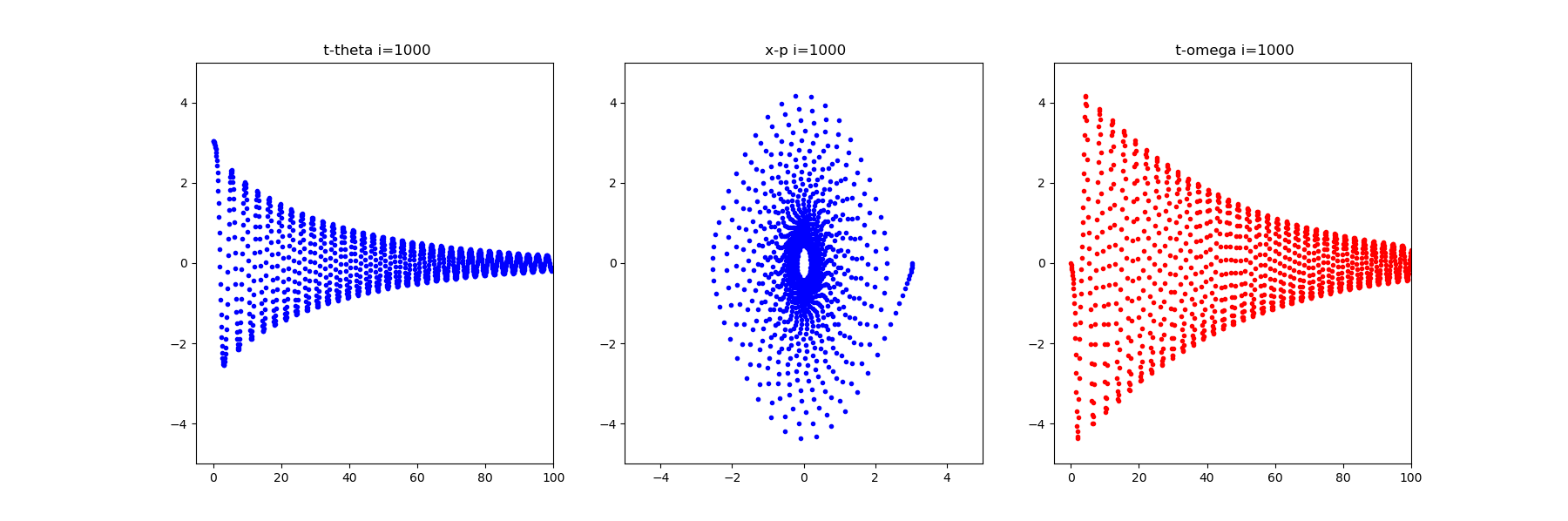
以下では、以前描画した常微分方程式の解の減衰振動をodeintで計算して描画しています。

減衰振動のアニメーションのコード

import matplotlib.animation as anm
import matplotlib.pyplot as plt
import numpy as np
from scipy.integrate import odeint, simps

def pend(y, t, b,c):
    theta, omega = y
    dydt = [omega, -c*omega-b*np.sin(theta)]
    return dydt

b = 5
c = 0.05
# 初期値y0=[theta0,omega0]
y0 = [np.pi - 0.1, 0.0]
# [0, 100]の範囲を1001の等間隔の時間tを生成
t = np.linspace(0, 100, 1001)
# odeint(関数,初期値,時間,関数の定数)
sol = odeint(pend, y0, t, args=(b,c))

fig = plt.figure(figsize = (18, 6))
ax1 = fig.add_subplot(1, 3, 1)
ax2 = fig.add_subplot(1, 3, 2)
ax3 = fig.add_subplot(1, 3, 3)

xdata, ydata = [], []
ln1, = ax2.plot(x[0], p[0], 'b.')
ln, = ax1.plot(t[0], sol[0,0], 'b.')
ln2, = ax3.plot(t[0], sol[0,1], 'r.')
ax2.set_xlim(-5, 5)
ax2.set_ylim(-5, 5)
ax1.set_xlim(-5, 100)
ax1.set_ylim(-5, 5)
ax3.set_xlim(-5, 100)
ax3.set_ylim(-5, 5)

def update(i, fig_title, A):
    y = sol[0:i, 0]
    y1 = sol[0:i, 1]
    ln1.set_data(x[0:i], p[0:i])
    ln.set_data(t[0:i], y)
    ln2.set_data(t[0:i], y1)
    ax2.set_title(fig_title +'x-p i=' + str(i))
    ax1.set_title(fig_title + 't-theta i=' + str(i))
    ax3.set_title(fig_title + 't-omega i=' + str(i))
    plt.pause(0.001)
    #return ln,

ani = anm.FuncAnimation(fig, update, fargs = ('Initial Animation! ', 2.0), \
    interval = 10, frames = 100)

ani.save("Sample_odeint.gif", writer = 'imagemagick')
plt.pause(10)

frames = 1000
ps = 10
s = 0 
for n in range(0,frames,ps):
    s+=ps
    num = s  #%100
    print(s, num) #,dataz)
    update(s,' ',A = 2.0)
    plt.pause(0.001)
fig.savefig("simple_odeint.png")
plt.close()

ani.save("Sample_odeint.gif", writer = 'imagemagick')の描画
※容量の都合で1000フレーム中の初めの200フレームを保存しています。

そして、最後のfig.savefig("simple_odeint.png")は以下のとおりです。
※もちろん画面上は時々刻々変化するアニメーションになっています。

・animationのmethods

この辺りで、気になるものに以下の関数群があります。
一応、表は載せておきますが、saveとjupyter notebook上で描画させるHTML以外はあまり使っている例は見つけられませんでした。
HTMLの使い方は以下のとおりです。
ちなみに、上記のsaveでもwriter指定していましたが、実はwriter = 'imagemagick'がインストールしていない場合は以下のエラーが出て代替で'matplotlib.animation.PillowWriter'を利用しており、指定ない場合も出力されます。
MovieWriter imagemagick unavailable; trying to use <class 'matplotlib.animation.PillowWriter'> instead.
また、ffmpegのインストールは出来ましたが、mp4出力は成功していません。

from matplotlib.animation import FFMpegWriter
# anim.save("anime_generator_savecount100_zorder_12_.mp4") #, writer=FFMpegWriter, dpi = 80)
writer = FFMpegWriter()
anim.save("anime_generator_savecount100_zorder_12_.mp4", writer=writer)

from IPython.display import HTML #for jupyter notebook
HTML(anim.to_jshtml())

Methods
__ init__(self, fig, func[, frames, ...])	Initialize self.
new_frame_seq(self)	Return a new sequence of frame information.
new_saved_frame_seq(self)	Return a new sequence of saved/cached frame information.
save(self, filename[, writer, fps, dpi, ...])	Save the animation as a movie file by drawing every frame.
to_html5_video(self[, embed_limit])	Convert the animation to an HTML5 tag.
to_jshtml(self[, fps, embed_frames, ...])	Generate HTML representation of the animation
new_frame_seq(self)	Return a new sequence of frame information.
new_saved_frame_seq(self)	Return a new sequence of saved/cached frame information.

まとめ

・アニメーションの定番FuncAnimation()関数で遊んでみた
・zorderの使い方と一般的なアニメーションを学んだ
・勝手に描画することにより、配列に格納した計算結果を使って、簡単にアニメーション出来ることも理解した

・gen_function()のyieldで間引きも出来るが、次回の宿題とする
・リサジュー図形のより一般的な描画もやりきれなかったので次回の宿題とする
・多くのシミュレーションが可能となるのでやってみようと思う