はじめに
第1回に引き続き時系列データを勉強していきます。
第1回(データの前処理)
第2回(LightGBMモデルの構築、Pycaretによるアンサンブルモデルの構築)
第3回(Prophetによる時系列モデルの構築、アンサンブル学習)
LightGBMモデル構築
まずはファーストチョイスでLightGBMによる回帰モデルを構築してみます(欠損値補完しなくていいから楽だし、LightGBM信者なので)。
第1回で前処理した訓練データ(train_df)とテストデータ(test_df)を使っていきます。まずはoptunaでハイパーパラメータの最適化を行います。
訓練データと検証データの分割はtrain_test_splitを使いましたが、時系列データなのでTimeSeriesSplitを使うのも手だと思います。どちらも試しましたが、train_test_splitでshuffleした方が精度が良かったです。
from sklearn.model_selection import KFold
import optuna.integration.lightgbm as lgb_op
from sklearn.model_selection import train_test_split
import lightgbm as lgb
from sklearn.metrics import mean_absolute_error as mae

df_train,df_val = train_test_split(train_data,test_size=0.2, shuffle=True, random_state=9)

col = 'y'
train_y = df_train[col]
train_x = df_train.drop(col,axis=1)

val_y = df_val[col]
val_x = df_val.drop(col,axis=1)

trains = lgb.Dataset(train_x,train_y)
valids = lgb.Dataset(val_x,val_y)

params = {
  'objective':'regression',
  'metric': 'mae',
  'force_row_wise' : True,
  'verbose': -1
}

tuner = lgb_op.LightGBMTunerCV(params, trains,num_boost_round=1000, optuna_seed=123, show_progress_bar=True)
tuner.run()

print('Best score:' ,{tuner.best_score})
print('Best params:')
print(tuner.best_params)
実行結果:
Best score: {5.079924313931009}
Best params:
{'objective': 'regression', 'metric': 'l1', 'force_row_wise': True, 'verbose': -1, 'feature_pre_filter': False, 'lambda_l1': 6.710378143115605, 'lambda_l2': 1.0164726750218338e-08, 'num_leaves': 31, 'feature_fraction': 0.5, 'bagging_fraction': 1.0, 'bagging_freq': 0, 'min_child_samples': 10}
最適化したハイパーパラメータを使ってLightGBMモデルを構築します。
model = lgb.train(tuner.best_params,
                  trains, valid_sets=[valids],
                  num_boost_round=10000,
                  callbacks=[lgb.early_stopping(stopping_rounds=100, verbose=True)]
                  )
実行結果:
Training until validation scores don't improve for 100 rounds
Early stopping, best iteration is:
[91] valid_0's l1: 5.27597
特徴量の重要度を確認します。
import matplotlib.pyplot as plt

importance = pd.DataFrame(model.feature_importance(), index=test_data.columns, columns=['importance'])

top30 = importance.nlargest(30, 'importance')

top30.sort_values(by='importance', ascending=True).plot(kind='barh', figsize=(10, 10))
plt.title('Feature Importances')
plt.xlabel('Importance')
plt.ylabel('Features')
plt.show()
実行結果:
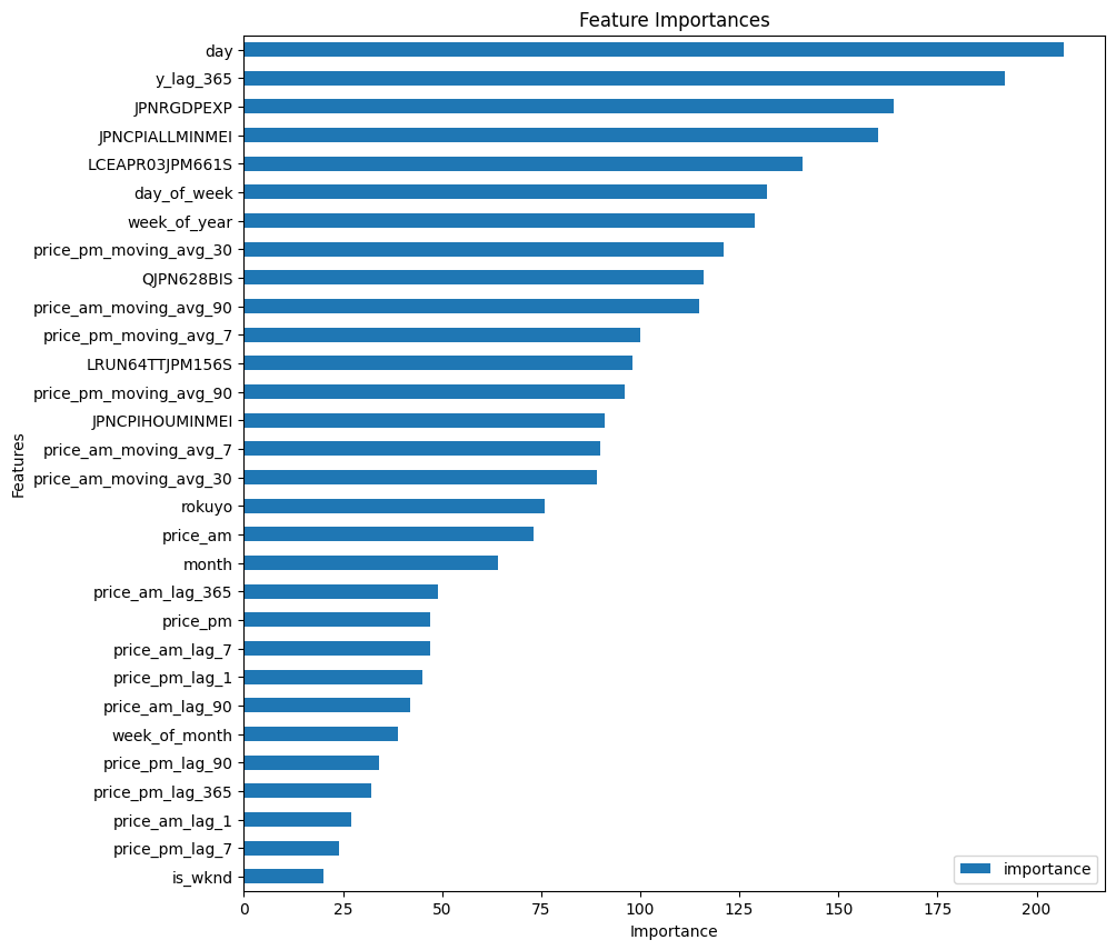
月よりも日が重要と認識されていますね。データを見ると、どうやら月末に引っ越し数が多いみたいです。
GDP成長率(JPNRGDPEXP)や消費者物価指数(JPNCPIALLMINMEI)も予測に大きく寄与しているので、景気が良いと引っ越し数が増えるのですかね(正の相関かまでは未確認なので逆かも)。特徴量として追加した甲斐がありました。
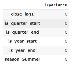
予測に寄与していない特徴量(重要度ゼロ)は削除して改めてモデルを構築します。
hreshold = 0

# 閾値以上の重要度を持つ特徴量を選択
selected_features = importance[threshold >=  importance['importance']]

selected_features
実行結果:
# 選択された特徴量の名前のリストを取得
selected_feature_names = selected_features.index.tolist()

# 元のデータセットから選択された特徴量のみを含む新しいデータフレームを作成
selected_feature_merged_df = merged_df.drop(columns=selected_feature_names)

selected_feature_train_data = selected_feature_merged_df[selected_feature_merged_df['is_train'] == 1].copy()
selected_feature_test_data = selected_feature_merged_df[selected_feature_merged_df['is_train'] == 0].copy()

selected_feature_train_data.drop(['is_train'], axis=1, inplace=True)
selected_feature_test_data.drop(['y','is_train'], axis=1, inplace=True)
先述と同様にoptunaでハイパーパラメータをチューニングしてLightGBMモデルを構築しました。
実行結果:
Training until validation scores don't improve for 100 rounds
Early stopping, best iteration is:
[81] valid_0's l1: 5.14548
若干精度があがりましたね!
可視化します。
prediction_train_data = pd.DataFrame(selected_feature_model.predict(selected_feature_train_data))
prediction_train_data.index = selected_feature_train_data.index
prediction_test_data = pd.DataFrame(selected_feature_model.predict(selected_feature_test_data))
prediction_test_data.index = selected_feature_test_data.index

plt.figure(figsize=(10, 6))
plt.plot(prediction_train_data.iloc[:,0], label='pridiction_train_data')
plt.plot(prediction_test_data.iloc[:,0], label='pridicttion_test_data')
plt.scatter(train_data.index, train_data['y'], color='gray', alpha=0.5, label='actual_y')
plt.xlabel('Date')
plt.ylabel('y')
plt.legend()
plt.show()
実行結果:
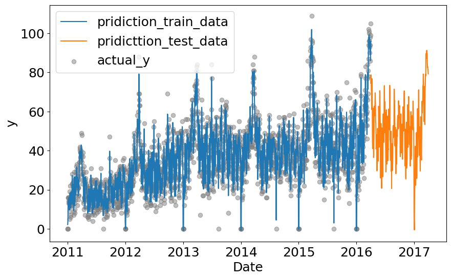
第1回で考察した感じ、引っ越し数は年々上昇傾向にあるはずですが、テストデータの予測を見るとLightGBMモデルがその傾向をとらえ切れていない気はしますね。
この予測結果を投稿したところ、
暫定評価(MAE):10.3442697
でした。これで400位後半くらいだったと思います。
Pycaretによるモデル構築
AutoMLで有名なPycaretでもモデルを構築してみます。Pycaretは欠損値の補完をしてくれるので、この後のProphetによる時系列モデルの構築において便利です(Prophetはテストデータは欠損値があっても良いが、訓練データは欠損値の補完が必要)。
データはLightGBMモデルで特徴量選択したデータを使用します。
import pandas as pd
import numpy as np

train_df = pd.read_csv('**/selected_feature_train_data.csv')
test_df = pd.read_csv('**/selected_feature_test_data.csv')
まずはsetupです。fold_strategyは時系列データなので'timeseries'にします(data_split_shuffle=Falseとしないとエラーになります)。
欠損値補完は"iterative"にしておきます。
from pycaret.regression import *

df_setup = setup(data=train_df,
                 target="y",
                 session_id=123,
                 fold_strategy= 'timeseries',
                 data_split_shuffle=False,
                 fold = 10,
                 imputation_type = "iterative",
                 numeric_iterative_imputer = "lightgbm",
                 normalize = False,
                 )
モデルを比較して、top3をbase_modelに格納しておきます。errors='raise'にしておくことでエラーが出た時点で計算が止まります。つまり、エラーが起きてるのに計算が走り続け、超時間待った挙句、空のリストが返されるという事態を防げます。
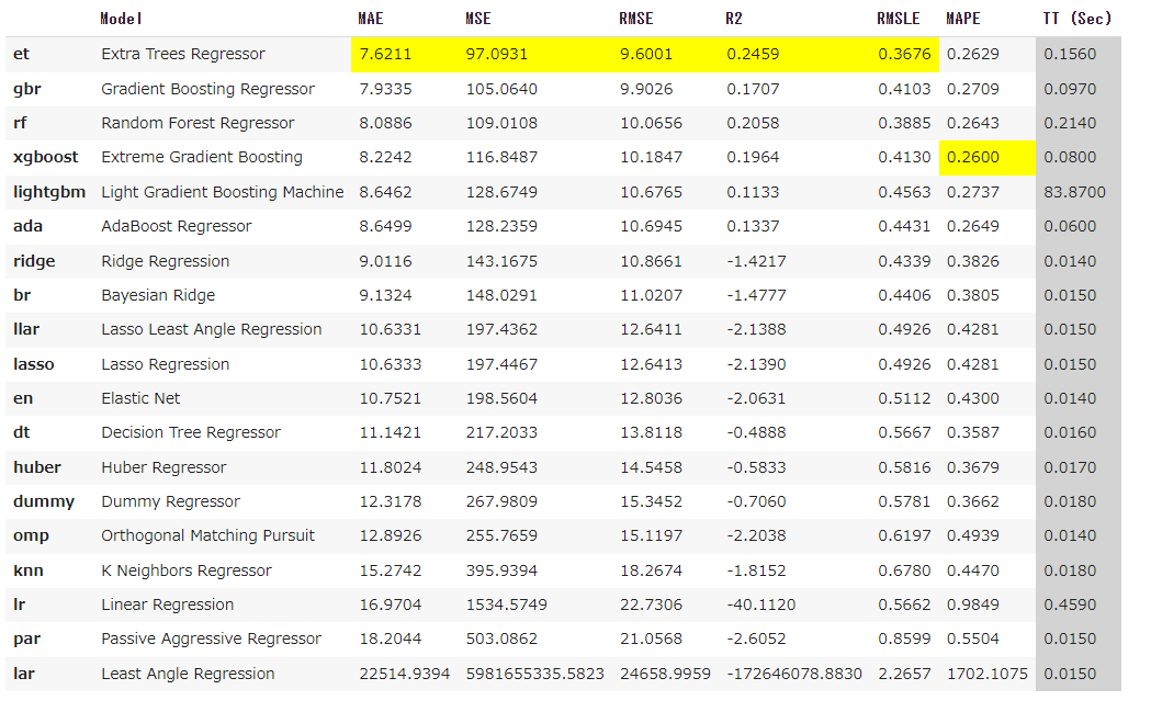
base_model = compare_models(sort='mae', errors='raise', n_select=3)
実行結果:
ブレンド、チューニング(重み調整)、最終モデル(検証データも含めた全データを使用したモデル)構築、テストデータの予測を行います。
blend  = blend_models(base_model)

tune_blend = tune_model(blend)

final_model = finalize_model(tune_blend)

prediction_test_data = predict_model(final_model, data = test_df)
訓練データと合わせて可視化します。
plt.figure(figsize = (10, 6))
plt.plot(prediction_train_data['prediction_label'], label = 'prediction_train')
plt.plot(sample_submission.iloc[:, 0], label = 'prediction_test')
plt.scatter(train_data.index, train_data['y'], label = 'actual_y', color='gray', alpha=0.5)
plt.xlabel('Date')
plt.ylabel('y')
plt.legend()
plt.show()
実行結果:
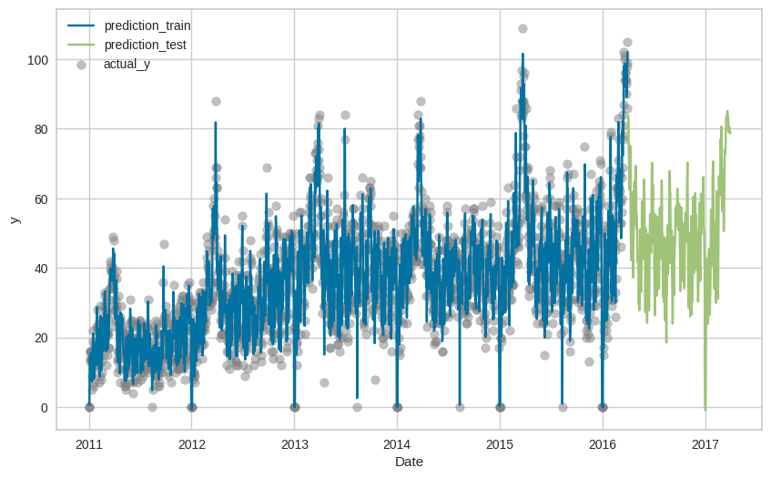
なんとなくLightGBMよりは訓練データにフィットしている気がしますが、テストデータを見るとやはり上昇トレンドをとらえ切れていないようです。
この予測結果を投稿したところ、
暫定評価(MAE):9.9571869
でした。LightGBMよりは多少精度があがりました。これで300位後半です。
おわりに
LightGBMとPycaretによる回帰モデルを構築してみました。いずれも訓練データにはそれなりにフィットしているようですが、上昇トレンドをとらえるのは難しいようです。
これが時系列用モデルだとどうなるか、次回をお楽しみに!('ω')ノ