この記事に関して
ここではpythonライブラリのblueqatを用いて量子数値積分を行っていこうと思います。
具体的な内容についてはここに述べています。
量子数値積分
積分値を量子コンピュータを用いて近似的に求めます。
今回は簡単に以下の積分を求めてみます。
\int_{0}^{1}\sin x dx \approx 0.45970
まずは近似値 $S(f)$ を以下で定義します。
S(f) = \sum_{x=0}^{2^n-1}\frac{1}{2^n}\sin\frac{x}{2^n} \ , \
\sum_{x=0}^{2^n-1}\frac{1}{2^n} = 1
確率密度関数は一様分布とします。
行列 P, R の作成
このとき $\mathcal{A}:=\mathcal{R}(\mathcal{P}\otimes\mathcal{I})$ は以下のようになります。
\mathcal{P}\left|0\right>_n := \sum_{x=0}^{2^n-1}\sqrt{\frac{1}{2^n}}\left|x\right>_n = H^{\otimes n}\left|x\right>_n\\
\mathcal{R}\left|x\right>_n\left|0\right>
:= \left|x\right>_n\left(\sqrt{\sin\frac{x}{2^n}}\left|0\right> + \sqrt{1-\sin\frac{x}{2^n}}\left|1\right>\right)
後半の部分はもう少し工夫して考えます。
$Rx$ ゲートでこの部分を近似してみます。
Rx(\theta)\left|0\right>
= \cos\left(\frac{\theta}{2}\right)\left|0\right>
+ \sin\left(\frac{\theta}{2}\right)\left|1\right>
= \sqrt{f(x)}\left|0\right>
+ \sqrt{1-f(x)}\left|1\right>
上の式が成り立つと仮定します。このとき $\left|0\right>$ の係数を比較して
\cos\left(\frac{\theta}{2}\right) = \sqrt{f(x)}\
\therefore \ \theta = 2\arccos\sqrt{f(x)}
このようになります。
この等式を頭に入れた上で以下の回路を考えます。
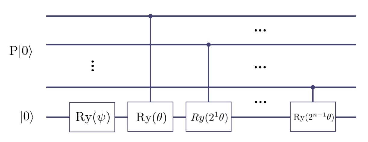
参考:https://arxiv.org/pdf/1904.10246.pdf
このとき各 $x$ に対して $\theta(x)$ は以下のようになります。
\theta(x) = \theta x + \psi
よってこの場合、 $\theta$ が一次なら求められることがわかります。
今回は
\theta(x) = 2\arccos\sqrt{f(x)} \approx \pi - 1 - \frac{1}{2^{n}}x =: \psi + \theta x
で一次近似しました。
これで $\mathcal{A}$ を作れました。
振幅増幅行列 Q の作成
$\mathcal{Q}$ の定義は以下で表します。
\mathcal{Q} := \mathcal{U}_{\Psi}\mathcal{U}_{\Psi_0}\\
\mathcal{U}_{\Psi_0} := I_n \otimes Z \\
\mathcal{U}_{\Psi} := \mathcal{A}\left(I_{n+1}-2\left|0\right>_{n+1}\left<0\right|_{n+1}\right)\mathcal{A}^{\dagger} \\
\left(I_{n+1}-2\left|0\right>_{n+1}\left<0\right|_{n+1} = X^{\otimes n+1}C^{n+1}ZX^{\otimes n+1}\right)
$\mathcal{A}$ が定義できているのでこれも容易に作ることができます。
全体図
最終的に以下の回路を作成します。
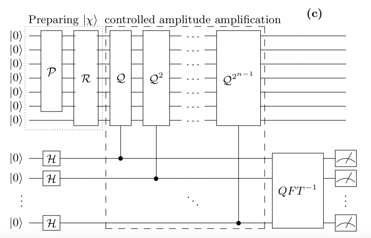
参考: https://arxiv.org/pdf/1805.00109.pdf
$C\mathcal{Q}$ ゲートや multi control ゲートについては制御トフォリゲートの構成を参考にしました。
実装
実際に回路を作ってみます。今回は $n=3$ で振幅推定も $m=3$ ビットとします。
# qubits
n = 3

# angle
phi = math.pi-1
theta = -1/(2^n)

# operator P, R (_R is the inverse)
P = Circuit().h[0,1,2]
R = Circuit().ry(phi)[3].cry(theta)[0,3].cry(2*theta)[1,3].cry(4*theta)[2,3]
_R = Circuit().cry(4*theta)[2,3].cry(2*theta)[1,3].cry(theta)[0,3].ry(phi)[3]

# A = R(P*I)
A = Circuit()+P+R
_A = Circuit()+_R+P

# multi control gates
def ccry(theta, c1, c2, t):
    c = Circuit().ccx[c1,c2,t].ry(-theta/2)[t].ccx[c1,c2,t].ry(theta/2)[t]
    return c

def cccx(c1, c2, c3, t):
    c = Circuit().cu2(0,math.pi)[c1,t].ccx[c1,c3,t].cu1(-math.pi/4)[c1,t].ccx[c1,c2,t]
    c.cu1(math.pi/4)[c1,t].ccx[c1,c3,t].cu1(-math.pi/4)[c1,t].ccx[c1,c2,t]
    c.cu1(math.pi/4)[c1,t].cu1(math.pi/4)[c1,c3].cu2(0,math.pi)[c1,t].ccx[c1,c2,c3]
    c.cu1(-math.pi/4)[c1,c3].cu1(math.pi/4)[c1,c2].ccx[c1,c2,c3]
    return c

def cQ(c):
    # cA_
    qc = (Circuit().cz[c,3]+ccry(4*theta,c,2,3)+ccry(2*theta,c,1,3)+ccry(theta,c,0,3)).cry(phi)[c,3]
    qc.cu2(0,math.pi)[c,0].cu2(0,math.pi)[c,1].cu2(0,math.pi)[c,2]

    # X*CZ*X
    (qc.cx[c,0].cx[c,1].cx[c,2].cu2(0,math.pi)[c,2]+cccx(c,0,1,2)).cu2(0,math.pi)[c,2].cx[c,0].cx[c,1].cx[c,2]

    # cA
    qc.cu2(0,math.pi)[c,0].cu2(0,math.pi)[c,1].cu2(0,math.pi)[c,2]
    qc.cry(phi)[c,3]+ccry(theta,c,0,3)+ccry(2*theta,c,1,3)+ccry(4*theta,c,2,3)

    return qc

# create circuit
qc = A.h[4,5,6]+cQ(4)+cQ(5)+cQ(5)+cQ(6)+cQ(6)+cQ(6)
qc.h[6].cu1(-math.pi/2)[6,5].h[5].cu1(-math.pi/4)[6,4].cu1(-math.pi/2)[5,4].h[4]

# observation
result = qc.m[4,5,6].run(shots=1000)
print(result.most_common())

label = [result.most_common()[i][0][4:] for i in range(len(result.most_common()))]
left = np.array([i for i in range(len(result.most_common()))])
height = np.array([result.most_common()[i][1]/1000 for i in range(len(result.most_common()))])

plt.title("Expectation", fontname="serif", fontsize=20)
plt.bar(left, height, tick_label=label, align="center", color="#414175", width=0.5)

# 結果
[('0000010', 243), ('0000110', 220), ('0000001', 200), ('0000111', 183),
('0000100', 54), ('0000101', 40), ('0000011', 35), ('0000000', 25)]
期待値は以下のようになります。(推定部分のみ取り出しました。)

もっとも期待値が高いものを $x$ として $S(f)$ を計算してみると
x = 2 \rightarrow \theta = \frac{\pi}{M}x = \frac{\pi}{4} \\
S(f) = \sin^2\theta = \frac{1}{2} = 0.5
それなりに近い値を出すことができました。
まとめ
今回はblueqatを用いて量子数値積分を実装しました。
参考文献
Amplitude Estimation without Phase Estimation
https://arxiv.org/pdf/1904.10246.pdf
制御トフォリゲートの構成
https://qiita.com/farcpan/items/9ccc300df7e6a3eadbfa