Pythonでテクスチャ解析をやる方法についてまとめました。

テクスチャ解析とは

テクスチャ解析は、画像の質感を数値化する画像処理の手法のひとつです。
画像の滑らかさ、粗さ、周期性などの度合いを数値化します。
テクスチャ解析についてはこちらの記事でまとめてくれています。

画像によってサイズやピクセルごとに取り得る値の範囲などが一定でないため、
これらの影響を少なくするためにテクスチャ解析前には画像の正規化が必要になります。

正規化するためのアルゴリズムには
- GLCM (Gray-Level Co-occurrence Matrix)
- GLSZM (Gray Level Size Zone Matrix)
- NGTDM (Neighbourhood Gray-Tone-Difference Matrix)
などがありますが、どれも画像を行列に変換することで正規化します。

今回はテクスチャ解析で最も基本的なGLCMをつかってみます。
GLCMの詳細についてはこちらの記事でまとめてくれています。

scikit-imageによるテクスチャ解析

今回は画像処理をおこなうPythonモジュールのひとつ、
scikit-imageを用いてテクスチャ解析をしてみます。
scikit-imageの公式ドキュメントを参考にしてやってみます。

環境

Windows 10
Python 3.8
scikit-image 0.18.1
jupyter lab

モジュールのインポート

import numpy as np
import pandas as pd
import matplotlib.pyplot as plt
from skimage.feature import greycomatrix, greycoprops
from skimage import data

データの読み込み

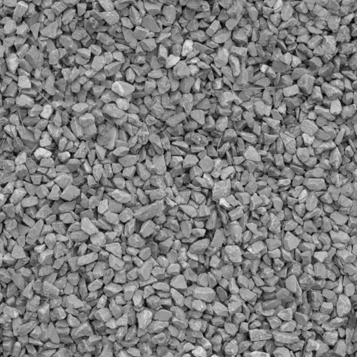
今回はscikit-imageに入っているサンプル画像gravelを使います。

image = data.gravel()
plt.imshow(image, cmap=plt.cm.gray)
plt.show()

パッチ画像の作成

PATCH_SIZEは今回は11にします。
locationsは作成するパッチの中心座標のリストです。

PATCH_SIZE = 11
locations = [(480, 460), (122, 203), (444, 192), (455, 453), (345, 145)]
patches = []
for loc in locations:
    patches.append(image[loc[0]-int(PATCH_SIZE/2):loc[0]+int(PATCH_SIZE/2+1),
                         loc[1]-int(PATCH_SIZE/2):loc[1]+int(PATCH_SIZE/2+1)])

作成したパッチを表示してみます。

fig = plt.figure(figsize=(10, 10))
for i, patch in enumerate(patches):
    ax = fig.add_subplot(3, len(patches), len(patches)*1 + i + 1)
    ax.imshow(patch, cmap=plt.cm.gray,vmin=0, vmax=255)
    ax.set_xlabel('location %d' % (i + 1))

パラメータ設定

ピクセル間の距離
ピクセル間の角度

今回は4つ右隣のピクセルとの関係をみる。

distances = [4]
angles = np.deg2rad([0]) # 度で入れラジアンに変換

どちらもリストだが1つ目しか反映されない？

GLCMの作成と各指標の計算

パッチごとにGLCMを求め、指標を算出する。

GLCM作成のイメージ図（distances = [1], angles = [0]の場合）

1つ右に隣接するピクセルとの関係をみるので、
(1,2)のペアは1つ、(4,4)のペアは3つあることがわかる。

scikit-imageで使用できるテクスチャ解析の指標は以下のもの。
似たような指標が多いですが求め方が異なります。
- contrast
- dissimilarity (不均一性)
- homogeneity (均一性)
- ASM (一様性)
- energy
- correlation

定義は以下の通り。PはGLCM。

contrast = []
dissimilarity = []
homogeneity = []
ASM = []
energy = []
correlation = []
for patch in patches:
    # GLCMを求める
    glcm = greycomatrix(patch, distances=distances, angles=angles, levels=256,
                        symmetric=True, normed=True)
    # 指標の算出
    contrast.append(greycoprops(glcm, 'contrast')[0, 0])
    dissimilarity.append(greycoprops(glcm, 'dissimilarity')[0, 0])
    homogeneity.append(greycoprops(glcm, 'homogeneity')[0, 0])
    ASM.append(greycoprops(glcm, 'ASM')[0, 0])
    energy.append(greycoprops(glcm, 'energy')[0, 0])
    correlation.append(greycoprops(glcm, 'correlation')[0, 0])

結果の確認

各locationの値を確認してみる。
energyはASMのルートをとっただけのものなので除外しました。

index = ['location {}'.format(i+1) for i in range(len(locations))]
df = pd.DataFrame({'contrast':contrast, 'dissimilarity':dissimilarity,
             'homogeneity':homogeneity, 'ASM':ASM, 'correlation':correlation}, index=index)
df

# 標準化
df = (df - df.min()) / (df.max() - df.min())
# バープロット
df.T.plot.bar(rot=0, figsize=(10, 6)).legend(bbox_to_anchor=(1.02, 0.3))

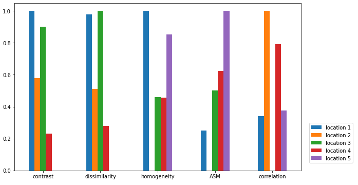
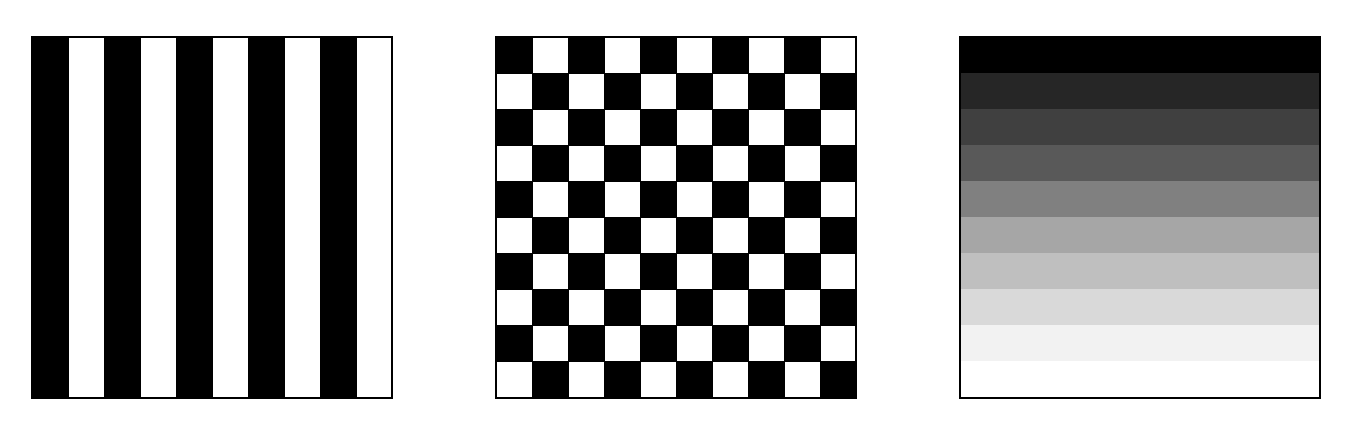
全体的に同色のパッチはcontrastやdissimilarityの値が小さくなります。
location 2は横縞模様に近く今回のパラメータではピクセル間の値の差が小さなるためcorrelationの値が大きくなっています。

最後に

今回は4つ左のピクセルとの関係を見てみました。
様々なテクスチャに対して距離と角度のパラメータを変えながらいろいろとやってみたいですね。

Pythonでテクスチャ解析をやってみる