最近流行りつつある科学計算処理向けの高水準言語「Julia」の基本操作をまとめていきます。
1.準備編
2.確率分布・仮説検定と可視化編
3.データフレーム操作編
chapter.2 確率分布
確率分布のパッケージがあったので、ほぼそのパッケージの紹介のような感じです。
R とはまた使用感が異なりますが、個人的にはこっちの方が直感的で好きです。
パッケージ:Distributions.jl
詳細:https://juliastats.org/Distributions.jl/stable/
1.パッケージ install
julia> import Pkg; Pkg.add("Distributions")
julia> using Distributions
この後、ランダムにデータを生成する場面がありますが、seed を固定したい場合は以下
julia> using Random
julia> Random.seed!([シード値])
2.確率分布オブジェクト
とりあえず名称そのま関数を実行してみるとわかる通り、デフォルトのパラメーターが設定されている。もちろん指定することもできる。
julia> Bernoulli()
Bernoulli{Float64}(p=0.5)
julia> Binomial()
Binomial{Float64}(n=1, p=0.5)
julia> Poisson()
Bernoulli{Float64}(p=0.5)

julia> Normal()
Normal{Float64}(μ=0.0, σ=1.0)
julia> Exponential()
Exponential{Float64}(θ=1.0)
julia> Gamma()
Gamma{Float64}(α=1.0, θ=1.0)
R で言う所の rnorm,pnrom,dnorm,qnormをやってみる。
julia> norm_dist = Normal(50.0, 10.0) # 確率分布オブジェクトを生成
Normal{Float64}(μ=50.0, σ=10.0)

julia> rand(norm_dist, 5) # 第二引数に size
5-element Array{Float64,1}:
 31.32159859451268
 76.52740439407731
 43.67613857974404
 49.230729489493726
 38.79220085610626

julia> rand(norm_dist, 5) # 第三引数で次元数
5×2 Array{Float64,2}:
 53.1482  33.9218
 40.4533  62.3337
 44.2832  45.7319
 48.4506  53.5824
 46.6584  39.3576

julia> pdf(norm_dist, 70)
0.005399096651318806

julia> cdf(norm_dist, 70)
0.9772498680518208

julia> quantile(norm_dist, 0.5)
50.0
パラメータを取り出す
julia> println("μ : ", norm_dist.μ)
μ : 50.0

julia> println("σ : ", norm_dist.σ)
σ : 10.0
配列の場合
julia> norm_dist = Normal() # とりあえずデータを生成
Normal{Float64}(μ=0.0, σ=1.0)

julia> array = rand(norm_dist, 5)
5-element Array{Float64,1}:
 -0.615182929965525
  0.3018546554695042
  0.43501627608696825
 -1.5087403568012359
 -1.5281565440128444
関数名称の直後に . を入れるだけ
julia> println(pdf.(norm_dist, array))
[0.33016473508059785, 0.3811750160113275, 0.36292534993233966, 0.1278257506789366, 0.12411214279395513]

julia> println(cdf.(norm_dist, array))
[0.26921695979105614, 0.6186185680364118, 0.6682246933064511, 0.06568257397844732, 0.06323683764142299]

julia> println(quantile.(norm_dist, 0.025 : 0.025 : 0.1))
[-1.9599639845400592, -1.6448536269514724, -1.439531470938456, -1.2815515655446004]
最尤推定
julia> norm_fitted = fit(Normal, array) # ここでfit
Normal{Float64}(μ=-0.5830417798446266, σ=0.8450652913045483)
確認してみる
julia> println(norm_fitted)
Normal{Float64}(μ=-0.5830417798446266, σ=0.8450652913045483)
パラメータを取り出す場合は先ほど同様...
julia> println(norm_fitted.μ)
-0.5830417798446266

julia> println(norm_fitted.σ)
0.8450652913045483
chapter.3 仮説検定
こちらも仮説検定パッケージがあったのでほぼその紹介になります。
パッケージ:HypothesisTests
詳細:https://hypothesistestsjl.readthedocs.io/en/latest/index.html
1.パッケージ install
julia> import Pkg; Pkg.add("HypothesisTests")
julia> using HypothesisTests, Distributions
2.とりあえずT検定
一標本
julia> x = rand(Normal(1,1), 10) # 適当にデータ生成

julia> ttest_object = OneSampleTTest(x, 0) # 第一引数にデータ、第二引数に帰無仮説
One sample t-test
-----------------
Population details:
    parameter of interest:   Mean
    value under h_0:         0
    point estimate:          1.332171049138298
    95% confidence interval: (0.7003, 1.9641)

Test summary:
    outcome with 95% confidence: reject h_0
    two-sided p-value:           0.0010

Details:
    number of observations:   10
    t-statistic:              4.7689293088672375
    degrees of freedom:       9
    empirical standard error: 0.27934384488805275
デフォルトでは両側なので、片側検定はpvalue関数を使う。tail で どっち側かを指定する
julia> println("right-side p-value : ", pvalue(ttest_object, tail=:right))
right-side p-value : 0.0005084438096162109
一応 Paired T
julia> before = rand(Normal(0,3), 10)
julia> after  = rand(Normal(1,1), 10)
julia> diff = after - before
julia> OneSampleTTest(diff, 0)
One sample t-test
-----------------
Population details:
    parameter of interest:   Mean
    value under h_0:         0
    point estimate:          0.661240160838284
    95% confidence interval: (-1.4651, 2.7876)

Test summary:
    outcome with 95% confidence: fail to reject h_0
    two-sided p-value:           0.4996

Details:
    number of observations:   10
    t-statistic:              0.70347237950898
    degrees of freedom:       9
    empirical standard error: 0.9399660599323403
等分散を仮定したT検定
julia> x1 = rand(Normal(0,1), 10)
julia> x2 = rand(Normal(1,1), 20)
julia> println(EqualVarianceTTest(x1, x2))
Two sample t-test (equal variance)
----------------------------------
Population details:
    parameter of interest:   Mean difference
    value under h_0:         0
    point estimate:          -1.3055004613593664
    95% confidence interval: (-1.9006, -0.7104)

Test summary:
    outcome with 95% confidence: reject h_0
    two-sided p-value:           0.0001

Details:
    number of observations:   [10,20]
    t-statistic:              -4.493473545511074
    degrees of freedom:       28
    empirical standard error: 0.29053257978196967
等分散を仮定しないT検定
julia> x1 = rand(Normal(0,3), 10)
julia> x2 = rand(Normal(1,1), 20)
julia> UnequalVarianceTTest(x1, x2)
Two sample t-test (unequal variance)
------------------------------------
Population details:
    parameter of interest:   Mean difference
    value under h_0:         0
    point estimate:          -1.8905345365179094
    95% confidence interval: (-4.01, 0.229)

Test summary:
    outcome with 95% confidence: fail to reject h_0
    two-sided p-value:           0.0750

Details:
    number of observations:   [10,20]
    t-statistic:              -1.9826311751666585
    degrees of freedom:       10.182596382128017
    empirical standard error: 0.9535482747359667
3.カイ二乗検定
とりあえずクロス集計表を作る
julia> p1 = 0.01
julia> n1 = 10000
julia> Ber1 = Bernoulli(p1)
julia> x1= rand(Ber1, n1)
julia> A = [sum(x1) n1-sum(x1)]
1×2 Array{Int64,2}:
 100  9900

julia> p2 = 0.015
julia> n2 = 8000
julia> Ber2 = Bernoulli(p2)
julia> x2= rand(Ber2, n2)
julia> B = [sum(x2) n2-sum(x2)]
1×2 Array{Int64,2}:
 138  7862

julia> X = [A ; B]
2×2 Array{Int64,2}:
 100  9900
 138  7862
検定
julia> ChisqTest(X)
Pearson's Chi-square Test
-------------------------
Population details:
    parameter of interest:   Multinomial Probabilities
    value under h_0:         [0.007345679012345679, 0.005876543209876543, 0.5482098765432099, 0.4385679012345679]
    point estimate:          [0.005555555555555556, 0.007666666666666666, 0.55, 0.43677777777777776]
    95% confidence interval: Tuple{Float64,Float64}[(0.0, 0.0132), (0.0, 0.0154), (0.5423, 0.5577), (0.4291, 0.4445)]

Test summary:
    outcome with 95% confidence: reject h_0
    one-sided p-value:           <1e-4

Details:
    Sample size:        18000
    statistic:          17.904808584847267
    degrees of freedom: 1
    residuals:          [-2.802226672320168, 3.132984663835462, 0.3243738295754118, -0.3626609665262763]
    std. residuals:     [-4.231407400008412, 4.231407400008412, 4.2314074000084645, -4.2314074000084645]
他の検定も概ね網羅している模様。
chapter.4 可視化
可視化のライブラリは色々ある模様。
ここでは StatsPlots.jl を使った可視化を行います。
またこの chapter は jupyter notebook 前提で書いています。
詳細:https://docs.juliaplots.org/latest/tutorial/
1.パッケージ install
import Pkg; Pkg.add("StatsPlots")
using StatsPlots
using Distributions
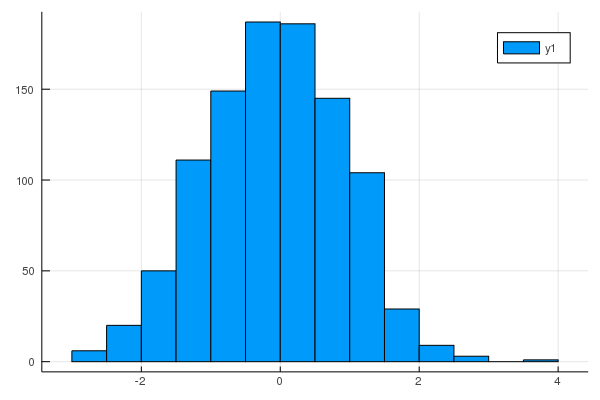
2.ヒストグラム
norm_dist = Normal()
norm = rand(norm_dist,1000)
StatsPlots.histogram(norm, bins=20)
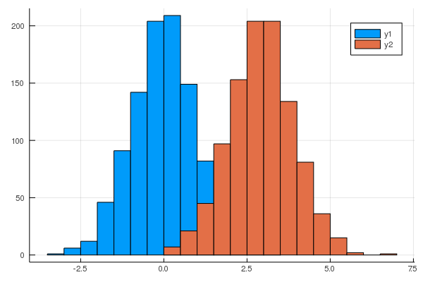
2つのヒストグラムを重ねる
norm_dist1 = Normal(0)
norm_dist2 = Normal(3)
norm1 = rand(norm_dist1,1000)
norm2 = rand(norm_dist2,1000)
StatsPlots.histogram([norm1 norm2])
! をつけると後から追加できる。
norm_dist1 = Normal(0)
norm_dist3 = Normal(5)
norm3 = rand(norm_dist3,1000)
StatsPlots.histogram!(norm3)
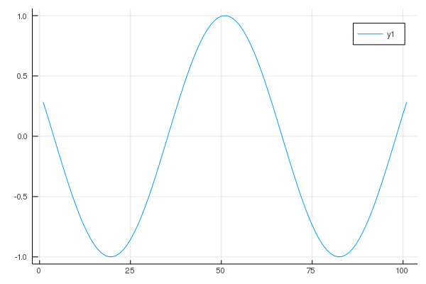
3.折れ線グラフ
coscurve = cos.(-5.0:0.1:5.0)
StatsPlots.plot(coscurve)
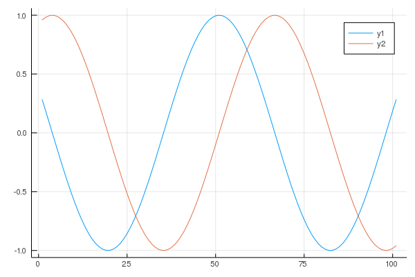
2つ重ねる
sincurve = sin.(-5.0:0.1:5.0)
StatsPlots.plot([coscurve sincurve])
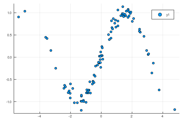
4.散布図
N = 100
norm_noize = rand(Normal(0,0.1) , N)
x = rand(Normal(0,2) , N)
y = sin.(x) .+ norm_noize
StatsPlots.plot(x,y,seriestype=:scatter)
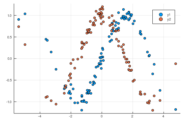
こちらも2つ重ねる
y2 = cos.(x) .+ norm_noize
StatsPlots.plot!(x,y2,seriestype=:scatter)
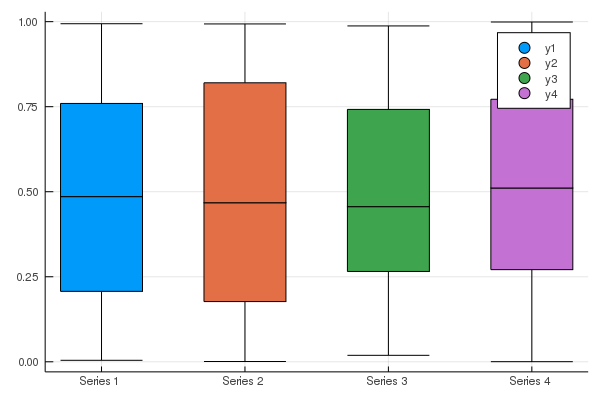
5.Boxプロット
y = rand(100,4) # Four series of 100 points each
StatsPlots.boxplot(["Series 1" "Series 2" "Series 3" "Series 4"],y,leg=false)
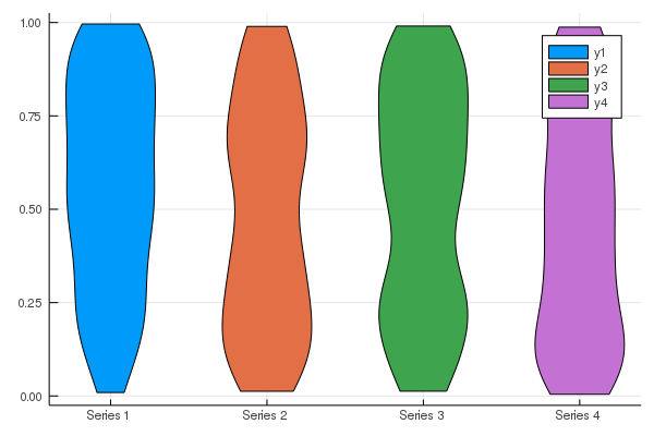
6.Violinプロット
(私は昆布グラフと呼んでいる。あんまり通じない)
y = rand(100,4)
StatsPlots.violin(["Series 1" "Series 2" "Series 3" "Series 4"],y)
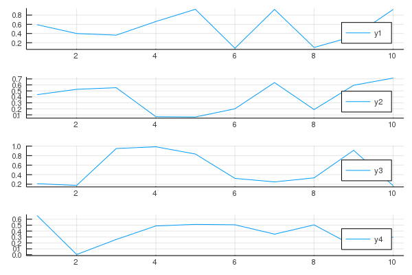
7.複数同時に表示
例1.
x = 1:10; y = rand(10,4)
StatPlots.plot(x, y, layout=(4, 1))
例2.
x = 1:10; y = rand(10, 4)
p1 = StatPlots.plot(x, y)
p2 = StatPlots.scatter(x, y)
p3 = StatPlots.plot(x, y)
p4 = StatPlots.histogram(x, y)
StatPlots.plot(p1, p2, p3, p4, layout=(2, 2), legend=false)
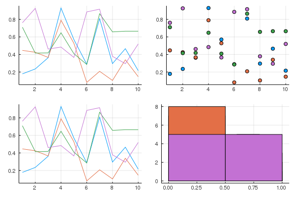
※棒グラフわからんかった...。
※散布図行列などの一斉に描画するタイプのものも見つからず...。
以上
次回は データフレーム操作の予定です。