はじめに
こんにちは、事業会社で働いているデータサイエンティストです。
本記事は、新しくでデータサイエンスチームにジョインした社員向けの研修資料です。
さて、「階層ベイズ」と聞いて、どんなものを思い浮かべるでしょうか?名前はなんだかかっこいいけれど、「結局何をやっているのかよくわからない」と感じる方も多いのではないでしょうか。
ここでは、機械学習の埋め込みモデル(参考リンク)を階層ベイズ化するような複雑な応用例ではなく、最もシンプルなケース:「平均値を推定する場面」で、同じグループ内の他の観測値から情報を借りるという現象を、実際のコードを通じて体験してみましょう。
さらに、データベースでよく使われる「マスターテーブル」のような概念も取り入れつつ、階層ベイズをどのように確率的プログラミングで実装できるのか、丁寧に解説していきます。
階層ベイズとは
階層ベイズは、「データの構造に応じて、パラメータにも階層的な構造を持たせる」というアプローチです。観測データがいくつかのグループに分かれているとき、それぞれのグループに専用のパラメータを割り当てつつ、それらのパラメータにも共通する上位の分布(ハイパーパラメータ)を導入するのが特徴です。
たとえば、ある市区町村における自動車保有台数の平均点を市区町村ごとに推定したいとします。サンプル数が多い市区町村もあれば、少ない市区町村もある中で、各市区町村の平均点を個別に推定してしまうと、データ数が少ない市区町村では推定が不安定になります。ここで階層ベイズを使うと、同じ都道府県内の市区町村の情報を借りてくることで、特にデータが少ないグループにおける推定精度を高めることができます。これを情報のプーリングと呼び、さらに三つの種類があります:
- 完全プーリング:すべての市区町村のデータをまとめて、共通の平均を推定する(差を無視)。
- 非プーリング:市区町村ごとにまったく独立に平均を推定する(情報を共有しない)。
- 部分プーリング:階層ベイズによるアプローチ。市区町村ごとの平均を持ちつつ、都道府県全体の平均からのズレとしてモデル化する(情報を共有しながら柔軟に差も認める)。
階層ベイズの魅力は、この部分プーリングによるバランス感覚にあります。特にサンプルサイズのばらつきが大きい現実のデータでは、非常に実用的な手法として活用されています。
以下のコードは、都道府県Aと都道府県Bに属する市区町村ごとに異なる「真の効果(city_effect)」を持つと仮定し、それに基づいた観測データを生成したものです。B県のc市のみサンプル数(N = 1泣)が極端に少ない状況をシミュレーションしています。
set.seed(12345)

city_effect_master <- tibble::tibble(
  tdfk = c("A", "A", "A", "A", "B", "B", "B", "B"),
  city = c("A_a", "A_b", "A_c", "A_d", "B_a", "B_b", "B_c", "B_d"),
  city_effect = c(1, 1, 1, 1, -1, -1, -1, -1)
)

df <- c(
  rep("A_a", 5000),
  rep("A_b", 5000),
  rep("A_c", 5000),
  rep("A_d", 5000),
  rep("B_a", 5000),
  rep("B_b", 5000),
  rep("B_c", 1),
  rep("B_d", 5000)
) |>
  tibble::tibble(
    city = _
  ) |>
  dplyr::left_join(
    city_effect_master, by = "city"
  ) |>
  dplyr::mutate(
    e = rnorm(dplyr::n()),
    y = city_effect + e
  )
要するに、A県のすべての市区町村の平均値は1、B県のすべての市区町村の平均値は-1という設定になっています。ただし、他の市区町村にはそれぞれ5,000件のデータがある一方で、B県のc市だけは1件しかサンプルがありません。このような場合、他のB県の市区町村から情報を借りてこないと、B_c市の平均を正確に推定するのは困難です。
このデータを用いて、Stanによる非階層モデルと階層ベイズモデルの実装を行い、「情報を借りてくる」という現象が推定結果にどのように表れるのかを実際に確かめていきます。
モデル実装
非階層モデル
非階層モデルの実装はとても簡単で、下記のベイズモデルを利用します。
まず、市区町村について
$$
\sigma_{city} \sim Inverse \space Gamma (0.01, 0.01)
$$
$$
\beta_{city} \sim Normal(0, \sigma_{city})
$$
次に、観測値iについて
$$
y_{i} \sim Normal(\beta_{city_{i}}, \sigma_{y})
$$
つまり、各観測値は、属している市区町村ごとに異なる平均パラメータ $\beta_{city_{i}}$ を持つ正規分布に従う、という構造になっています。また、この非階層モデルでは、市区町村ごとの $\beta$ は互いに完全に独立しており、情報を共有していません。
実装用のコードはこちらになります:
data {
  int N;
  int city_type;

  array[N] int city;
  vector[N] y;
}
parameters {
  vector<lower=0>[city_type] sigma_city;
  vector[city_type] beta_city;

  real<lower=0> sigma_y;
}
model {
  sigma_city ~ inv_gamma(0.01, 0.01);
  beta_city ~ normal(0, sigma_city);

  sigma_y ~ inv_gamma(5, 5);

  y ~ normal(beta_city[city], sigma_y);
}
階層モデル
階層モデルの場合、まず都道府県について
$$
\sigma_{tdfk} \sim Inverse \space Gamma(0.01, 0.01)
$$
$$
\beta_{tdfk} \sim Normal(0, \sigma_{tdfk})
$$
$$
\sigma_{city} \sim Inverse \space Gamma(0.01, 0.01)
$$
$\beta_{tdfk}$は都道府県レベルの平均パラメータです。$\sigma_{city}$は都道府県内の市区町村の平均パラメータにどれほどの変動・ばらつきを許すかを決めるパラメータで、実際のデータを用いて推定されます。
続いて、市区町村について
$$
\beta_{city} \sim Normal(\beta_{tdfk_{city}}, \sigma_{city_{city}})
$$
要するに、市区町村ごとの平均パラメータは、その市区町村が属する都道府県の平均パラメータを平均とし、都道府県内の市区町村間のばらつきを表すパラメータを分散とする正規分布に従う、という構造です。
非階層モデルでは、市区町村の平均パラメータは完全に独立に推定されますが、階層モデルでは、同じ都道府県に属する市区町村は共通の都道府県レベルのパラメータを基に生成されるため、同一都道府県内の市区町村同士に統計的な関連性が生まれます。
実装用のコードはこちらになります:
data {
  int N;
  int tdfk_type;
  int city_type;

  array[city_type] int tdfk_city_master_tdfk;

  array[N] int city;
  vector[N] y;
}
parameters {
  vector<lower=0>[tdfk_type] sigma_tdfk;
  vector[tdfk_type] beta_tdfk;

  vector<lower=0>[tdfk_type] sigma_city;
  vector[city_type] beta_city;

  real<lower=0> sigma_y;
}
model {
  sigma_tdfk ~ inv_gamma(0.01, 0.01);
  beta_tdfk ~ normal(0, sigma_tdfk);

  sigma_city ~ inv_gamma(0.01, 0.01);
  beta_city ~ normal(beta_tdfk[tdfk_city_master_tdfk], sigma_city[tdfk_city_master_tdfk]);

  sigma_y ~ inv_gamma(5, 5);

  y ~ normal(beta_city[city], sigma_y^2);
}
ここのtdfk_city_master_tdfkが重要です。SQLで説明するため、まず下記のtdfk_city_tbをご確認ください:
| 市区町村ID | 都道府県ID |
|---|---|
| 1 | 1 |
| 2 | 1 |
| 3 | 1 |
| 4 | 1 |
| 5 | 2 |
| 6 | 2 |
| 7 | 2 |
| 8 | 2 |
よくある都道府県市区町村マスターですね。
このテーブルの都道府県ID列はtdfk_city_master_tdfkとしてStanに渡せば十分です。市区町村IDもStanに渡すことは可能ですが、1から8までの連番に過ぎないため、Stan内でforループを使って生成したほうが効率的です。
前処理
まず、city_masterを作り、市区町村の番号を付与して、元のデータにleft joinでくっつけます:
city_master <- df |>
  dplyr::select(city) |>
  dplyr::distinct() |>
  dplyr::mutate(
    city_id = dplyr::n() |>
      seq_len()
  )

df_with_id <- df |>
  dplyr::left_join(city_master, by = "city")
次に、Stanに渡すためにデータをlist型に整形します:
data_list_simple <- list(
  N = nrow(df_with_id),
  city_type = nrow(city_master),
  city = df_with_id$city_id,
  y = df_with_id$y
)
さて、モデルをコンパイルして
m_simple_init <- cmdstanr::cmdstan_model("simple_bayes.stan")
変分推論によるベイズ推定を実施します:
> m_simple_estimate <- m_simple_init$variational(
     data = data_list_simple
 )
------------------------------------------------------------
EXPERIMENTAL ALGORITHM:
  This procedure has not been thoroughly tested and may be unstable
  or buggy. The interface is subject to change.
------------------------------------------------------------
Gradient evaluation took 0.000432 seconds
1000 transitions using 10 leapfrog steps per transition would take 4.32 seconds.
Adjust your expectations accordingly!
Begin eta adaptation.
Iteration:   1 / 250 [  0%]  (Adaptation)
Iteration:  50 / 250 [ 20%]  (Adaptation)
Iteration: 100 / 250 [ 40%]  (Adaptation)
Iteration: 150 / 250 [ 60%]  (Adaptation)
Iteration: 200 / 250 [ 80%]  (Adaptation)
Iteration: 250 / 250 [100%]  (Adaptation)
Success! Found best value [eta = 0.1].
Begin stochastic gradient ascent.
  iter             ELBO   delta_ELBO_mean   delta_ELBO_med   notes
   100       -85135.519             1.000            1.000
   200       -81274.185             0.524            1.000
   300       -69616.120             0.405            0.167
   400       -65020.660             0.321            0.167
   500       -59105.105             0.277            0.100
   600       -56265.035             0.239            0.100
   700       -53316.602             0.213            0.071
   800       -51802.154             0.190            0.071
   900       -50901.946             0.171            0.055
  1000       -50512.748             0.155            0.055
  1100       -50136.197             0.055            0.050
  1200       -49986.970             0.051            0.050
  1300       -49809.965             0.035            0.029
  1400       -49754.061             0.028            0.018
  1500       -49651.109             0.018            0.008   MEDIAN ELBO CONVERGED
Drawing a sample of size 1000 from the approximate posterior...
COMPLETED.
Finished in  0.8 seconds.
一瞬で終わりました!
最後に、結果を整形して保存します:
m_simple_summary <- m_simple_estimate$summary()
続いて、階層ベイズモデルに入りますが、まず都道府県マスターと都道府県と市区町村の対照関係を表すマスターテーブルも作成します:
tdfk_master <- city_effect_master |>
  dplyr::select(tdfk) |>
  dplyr::distinct() |>
  dplyr::mutate(
    tdfk_id = dplyr::n() |>
      seq_len()
  )


tdfk_city_master <- city_effect_master |>
  dplyr::select(tdfk, city) |>
  dplyr::left_join(city_master, by = "city") |>
  dplyr::left_join(tdfk_master, by = "tdfk")
次に、Stanに渡すためにデータをlist型に整形します:
data_list_hier <- list(
  N = nrow(df_with_id),
  tdfk_type = nrow(tdfk_master),
  city_type = nrow(city_master),

  tdfk_city_master_tdfk = tdfk_city_master$tdfk_id,

  city = df_with_id$city_id,
  y = df_with_id$y
)
モデルをコンパイルして
m_hier_init <- cmdstanr::cmdstan_model("hierarchy_bayes.stan")
同じく変分推論によるベイズ推定を実施します:
> m_hier_estimate <- m_hier_init$variational(
     data = data_list_hier
 )
------------------------------------------------------------
EXPERIMENTAL ALGORITHM:
  This procedure has not been thoroughly tested and may be unstable
  or buggy. The interface is subject to change.
------------------------------------------------------------
Gradient evaluation took 0.000424 seconds
1000 transitions using 10 leapfrog steps per transition would take 4.24 seconds.
Adjust your expectations accordingly!
Begin eta adaptation.
Iteration:   1 / 250 [  0%]  (Adaptation)
Iteration:  50 / 250 [ 20%]  (Adaptation)
Iteration: 100 / 250 [ 40%]  (Adaptation)
Iteration: 150 / 250 [ 60%]  (Adaptation)
Iteration: 200 / 250 [ 80%]  (Adaptation)
Success! Found best value [eta = 1] earlier than expected.
Begin stochastic gradient ascent.
  iter             ELBO   delta_ELBO_mean   delta_ELBO_med   notes
   100      -556205.836             1.000            1.000
   200      -118501.964             2.347            3.694
   300       -54400.960             1.957            1.178
   400       -49808.831             1.491            1.178
   500       -49527.511             1.194            1.000
   600       -49560.747             0.995            1.000
   700       -49537.802             0.853            0.092
   800       -49497.828             0.746            0.092
   900       -49538.994             0.664            0.006   MEDIAN ELBO CONVERGED
Drawing a sample of size 1000 from the approximate posterior...
COMPLETED.
Finished in  0.6 seconds.
こちらも一瞬で終わりました!
最後に、結果を整形して保存します:
m_hier_summary <- m_hier_estimate$summary()
結果の可視化
ここでは、実際に事後分布を可視化して、二つのモデルの推定結果の違いを確認しましょう:
g_simple <- m_simple_estimate$draws("beta_city") |>
  tibble::as_tibble() |>
  tibble::rowid_to_column(var = "sample_id") |>
  dplyr::mutate(
    dplyr::across(
      dplyr::everything(),
      ~ as.numeric(.)
    )
  ) |>
  tidyr::pivot_longer(!sample_id, names_to = "city", values_to = "value") |>
  ggplot2::ggplot() +
  ggplot2::geom_density(ggplot2::aes(x = value, fill = city), alpha = 0.3) +
  ggplot2::ggtitle("非階層モデル") +
  ggplot2::theme_gray(base_family = "HiraKakuPro-W3") +
  ggplot2::scale_x_continuous(
    breaks = seq(-1.5, 1.5, by = 0.5),
    limits = c(-1.5, 1.5)
  )


g_hier <- m_hier_estimate$draws("beta_city") |>
  tibble::as_tibble() |>
  tibble::rowid_to_column(var = "sample_id") |>
  dplyr::mutate(
    dplyr::across(
      dplyr::everything(),
      ~ as.numeric(.)
    )
  ) |>
  tidyr::pivot_longer(!sample_id, names_to = "city", values_to = "value") |>
  ggplot2::ggplot() +
  ggplot2::geom_density(ggplot2::aes(x = value, fill = city), alpha = 0.3) +
  ggplot2::ggtitle("階層モデル") +
  ggplot2::theme_gray(base_family = "HiraKakuPro-W3") +
  ggplot2::scale_x_continuous(
    breaks = seq(-1.5, 1.5, by = 0.5),
    limits = c(-1.5, 1.5)
  )


gridExtra::grid.arrange(g_simple, g_hier, ncol = 1)
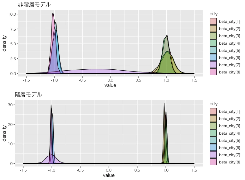
まず、観測値が1件しかないbeta_city[7]に注目してください。非階層モデルでは、事後分布のばらつきが非常に大きく、真の値である-1ではなく0付近に最も高い確率質量があり、符号(正か負か)すら統計的に有意とは言えないことが視覚的にわかります。
一方、階層モデルでは、ばらつきは他の市区町村と比べて依然として大きいものの、非階層モデルと比べれば劇的に小さくなっており、分布の中心も真の値である-1付近にあります。これは、階層ベイズモデルにおいてbeta_city[7]が同じ都道府県内の他の市区町村データから情報を借りていることを示しています。
もちろん、同じ都道府県内の情報を借りているのは B県c市(観測値1件)だけではありません。視覚的に確認できるように、他の市区町村の係数分布も非階層モデルに比べてばらつきが小さくなり、真の値の周辺に集中しています。つまり、各市区町村の推定には、自身の5000件のデータに加えて、同じ都道府県の他の市区町村からの情報が統計的に活用されており、実質的に使用されている情報量が増えていることを意味します。
結論
いかがでしょうか?
このように、階層ベイズモデルを用いることで、データ数が少ないケース(ここでは市区町村)に対しても、同じ都道府県内の他の市区町村データから情報を借りることにより、より精度の高い推定が可能になります。
もちろん、実際のデータにおいては、同じ都道府県内の市区町村がまったく同じ係数を持つことは稀です。しかし、階層ベイズモデルではこの関係性を、データによって覆すことが可能なソフトな仮定として扱います。
言い換えれば、「データが少ない段階では、同じ都道府県内の他の市区町村と大きくは違わないだろう」というベイズ的な帰無仮説(あくまで便宜的な呼び方です)を初期設定として置き、実際の観測データが増え、その仮説が適切でないと示された場合には、仮定から逸脱し、独自の値を持つことを許容するという設計です。
このような階層ベイズの性質については、別の機会にシミュレーションを通じてさらに具体的にお見せしたいと思います。
最後に、私たちと一緒にデータサイエンスの力を使って社会を改善していきたい方はぜひこちらのページをご確認ください: