はじめに
こんにちは、事業会社で働いているデータサイエンティストです。
階層ベイズは柔軟にモデルにドメイン知識を教える方法だと以前の記事で説明しました。
では、テキストアズデータ(自然言語処理)で有名なword2vec(Mikolov et al. 2013とRudolph et al. 2016)に階層ベイズの構造を入れたらどうなるか?というのを今回の記事で可視化して比較します!
データ説明
今回の記事では、下記の消費者購買情報データセットを利用します。
このように、ユーザーが何を買ったのかを記録したデータです:
> purchase_data <- readr::read_csv("events.csv")
Rows: 885129 Columns: 9
── Column specification ───────────────────────────────────────────────────────────────────────────────────────────────────────────────────────────────────────────────────
Delimiter: ","
chr (5): event_time, event_type, category_code, brand, user_session
dbl (4): product_id, category_id, price, user_id

ℹ Use `spec()` to retrieve the full column specification for this data.
ℹ Specify the column types or set `show_col_types = FALSE` to quiet this message.
> purchase_data
# A tibble: 885,129 × 9
   event_time              event_type product_id category_id category_code                 brand        price user_id user_session
   <chr>                   <chr>           <dbl>       <dbl> <chr>                         <chr>        <dbl>   <dbl> <chr>
 1 2020-09-24 11:57:06 UTC view          1996170     2.14e18 electronics.telephone         NA           31.9  1.52e18 LJuJVLEjPT
 2 2020-09-24 11:57:26 UTC view           139905     2.14e18 computers.components.cooler   zalman       17.2  1.52e18 tdicluNnRY
 3 2020-09-24 11:57:27 UTC view           215454     2.14e18 NA                            NA            9.81 1.52e18 4TMArHtXQy
 4 2020-09-24 11:57:33 UTC view           635807     2.14e18 computers.peripherals.printer pantum      114.   1.52e18 aGFYrNgC08
 5 2020-09-24 11:57:36 UTC view          3658723     2.14e18 NA                            cameronsino  15.9  1.52e18 aa4mmk0kwQ
 6 2020-09-24 11:57:59 UTC view           664325     2.14e18 construction.tools.saw        carver       52.3  1.52e18 vnkdP81DDW
 7 2020-09-24 11:58:23 UTC view          3791349     2.14e18 computers.desktop             NA          215.   1.52e18 J1t6sIYXiV
 8 2020-09-24 11:58:24 UTC view           716611     2.14e18 computers.network.router      d-link       53.1  1.52e18 kVBeYDPcBw
 9 2020-09-24 11:58:25 UTC view           657859     2.14e18 NA                            NA           34.2  1.52e18 HEl15U7JVy
10 2020-09-24 11:58:31 UTC view           716611     2.14e18 computers.network.router      d-link       53.1  1.52e18 F3VB9LYp39
# ℹ 885,119 more rows
# ℹ Use `print(n = ...)` to see more rows
このデータの中の商品を「単語」にして、ベイズword2vecモデルで分析し、学習された商品の分散表現が階層ベイズ構造によってどのように変わるかを可視化します。
テキストアズデータ分析の本質は、とあるアイテムの出現予測や何かしらのクラスタリングなどのタスクであって、対象が単語であろうと、商品であろうと、実質的には同じです。
実はテキストアズデータで有名なLDAの論文(Blei et al. 2003)でも、トピックモデルをユーザーの行動解析に利用する事例が紹介されました(p. 1014あたり)。
詳細はこちらの2本の記事を確認してください:
ここで協調しておきたいのは、本記事は商品を対象に分析しますが、モデルの拡張性と説明しやすさの観点から、一部「単語」という表現を使うこともあります。
モデル説明
負例サンプリングの概念
まず、word2vecや他の指数型分布族埋め込み(Rudolph et al. 2016、呉 2023)では、単語やアイテムの分散表現を学習するために、負例サンプリングを利用することが多いです。
具体的な説明は下記の記事を参考してください
要するに、普通のデータにデタラメの偽物データを混入して、モデルに本物か偽物か(本物フラグ)を判別させることで学習させます。
普通のベイズword2vec
まずは、階層構造のないベイズword2vecの構造を説明します。
定式化
- 全ての単語wについて
$$ sigma_{w} \sim Gamma(0.1, 0.1) $$
$$ word\space embedding_{w} \sim Normal(0,sigma_{w}) $$
$$ word\space context_{w} \sim Normal(0,1) $$
- 全ての本物フラグ判定iについて
$$ \eta = word\space embedding_{word_{i}} '* \Sigma_{c \in 文脈_{i}} word\space context_{c} $$
$$ 本物フラグ \sim Bernoulli(logit(\eta)) $$
要するに、単語がデタラメかどうかは、その単語の分散表現(word embedding)とその単語の周囲の単語の分散表現(word context)の和の内積で表現できるという定式化です。
Stanでの実装
このようにStanで実装できます:
functions {
  real partial_sum_lpmf(
    array[] int flag,
    int start, int end,

    array[] int word,
    array[] int word_lead_1,
    array[] int word_lag_1,

    array[] vector word_embedding,
    array[] vector word_context
  ){
    vector[end - start + 1] lambda;
    int count = 1;
    for (i in start:end){
      lambda[count] = word_embedding[word[i]] '* (word_context[word_lead_1[i]] + word_context[word_lag_1[i]]);
      count += 1;
    }
    return bernoulli_logit_lupmf(flag | lambda);
  }
}
data {
  int<lower=1> N;
  int<lower=1> M;
  int<lower=1> word_type;

  array[N] int<lower=1,upper=word_type> word;
  array[N] int<lower=1,upper=word_type> word_lead_1;
  array[N] int<lower=1,upper=word_type> word_lag_1;
  array[N] int<lower=0,upper=1> flag;

  int<lower=0> val_N;
  array[val_N] int<lower=1,upper=word_type> val_word;
  array[val_N] int<lower=1,upper=word_type> val_word_lead_1;
  array[val_N] int<lower=1,upper=word_type> val_word_lag_1;
  array[val_N] int<lower=0,upper=1> val_flag;
}
parameters{
  vector<lower=0>[word_type] word_sigma;
  array[word_type] vector[M] word_embedding;
  array[word_type] vector[M] word_context;
}
model{
  word_sigma ~ gamma(0.1, 0.1);

  for (w in 1:word_type){
    word_embedding[w] ~ normal(0, word_sigma[w]);
    word_context[w] ~ normal(0, 1);
  }

  int grainsize = 1;

  target += reduce_sum(
    partial_sum_lupmf, flag, grainsize,

    word,
    word_lead_1,
    word_lag_1,

    word_embedding,
    word_context
  );
}
generated quantities {
  real F1_score;
  {
    array[val_N] int predicted;
    int TP = 0;
    int FP = 0;
    int FN = 0;

    for (i in 1:val_N){
      predicted[i] = bernoulli_logit_rng(word_embedding[val_word[i]] '* (word_context[val_word_lead_1[i]] + word_context[val_word_lag_1[i]]));
      if (val_flag[i] == 1 && predicted[i] == 1){
        TP += 1;
      }
      else if (val_flag[i] == 0 && predicted[i] == 1){
        FP += 1;
      }
      else if (val_flag[i] == 1 && predicted[i] == 0){
        FN += 1;
      }
    }
    F1_score = (2 * TP) * 1.0/(2 * TP + FP + FN);
  }
}
階層ベイズ化word2vec
階層ベイズ化したモデルはこのような形で定式化されます。
定式化
- 全てのカテゴリkについて
$$ category \space embedding_{k} \sim Normal(0,1) $$
- 全ての単語wについて
$$ sigma_{w} \sim Gamma(0.1, 0.1) $$
$$ word\space embedding_{w} \sim Normal(category \space embedding_{カテゴリ_{w}},sigma_{w}) $$
$$ word\space context_{w} \sim Normal(0,1) $$
- 全ての本物フラグ判定iについて
$$ \eta = word\space embedding_{word_{i}} '* \Sigma_{c \in 文脈_{i}} word\space context_{c} $$
$$ 本物フラグ \sim Bernoulli(logit(\eta)) $$
普通のベイズword2vecとの一番大きな違いはカテゴリの存在です。全ての単語が何かしらのカテゴリに属しており、その分散表現(word embedding)がカテゴリの分散表現(category embedding)を平均ベクトルとする正規分布に従うと仮定します。
これを今回利用するデータで説明すると、パソコンはMacでもWindowsでも、結局同じパソコンなので、同じような形で消費者に買われる(充電と一緒に買われる、パソコンケースと一緒に買われる、など)。よって、MacとWindowsの分散表現はパソコンカテゴリの分散表現付近に推移しているはずです。
適切かはともかく、このドメイン知識は数学的に階層ベイズで表現できます。
Stanでの実装
このようにStanで実装できます:
functions {
  real partial_sum_lpmf(
    array[] int flag,
    int start, int end,

    array[] int word,
    array[] int word_lead_1,
    array[] int word_lag_1,

    array[] vector word_embedding,
    array[] vector word_context
  ){
    vector[end - start + 1] lambda;
    int count = 1;
    for (i in start:end){
      lambda[count] = word_embedding[word[i]] '* (word_context[word_lead_1[i]] + word_context[word_lag_1[i]]);
      count += 1;
    }
    return bernoulli_logit_lupmf(flag | lambda);
  }
}
data {
  int<lower=1> N;
  int<lower=1> M;
  int<lower=1> word_type;
  int<lower=1> category_type;

  // category master
  array[word_type] int<lower=1,upper=word_type> category_master_category;

  array[N] int<lower=1,upper=word_type> word;
  array[N] int<lower=1,upper=word_type> word_lead_1;
  array[N] int<lower=1,upper=word_type> word_lag_1;
  array[N] int<lower=0,upper=1> flag;

  int<lower=0> val_N;
  array[val_N] int<lower=1,upper=word_type> val_word;
  array[val_N] int<lower=1,upper=word_type> val_word_lead_1;
  array[val_N] int<lower=1,upper=word_type> val_word_lag_1;
  array[val_N] int<lower=0,upper=1> val_flag;
}
parameters{
  array[category_type] vector[M] category_embedding;
  vector<lower=0>[word_type] word_sigma;
  array[word_type] vector[M] word_embedding;
  array[word_type] vector[M] word_context;
}
model{
  for (c in 1:category_type){
    category_embedding[c] ~ normal(0, 1);
  }

  word_sigma ~ gamma(0.1, 0.1);

  for (w in 1:word_type){
    word_embedding[w] ~ normal(category_embedding[category_master_category[w]], word_sigma[w]);
    word_context[w] ~ normal(0, 1);
  }

  int grainsize = 1;

  target += reduce_sum(
    partial_sum_lupmf, flag, grainsize,

    word,
    word_lead_1,
    word_lag_1,

    word_embedding,
    word_context
  );
}
generated quantities {
  real F1_score;
  {
    array[val_N] int predicted;
    int TP = 0;
    int FP = 0;
    int FN = 0;

    for (i in 1:val_N){
      predicted[i] = bernoulli_logit_rng(word_embedding[val_word[i]] '* (word_context[val_word_lead_1[i]] + word_context[val_word_lag_1[i]]));
      if (val_flag[i] == 1 && predicted[i] == 1){
        TP += 1;
      }
      else if (val_flag[i] == 0 && predicted[i] == 1){
        FP += 1;
      }
      else if (val_flag[i] == 1 && predicted[i] == 0){
        FN += 1;
      }
    }
    F1_score = (2 * TP) * 1.0/(2 * TP + FP + FN);
  }
}
前処理
まずは、マスター系のテーブルを作成します:
item_master <- purchase_data |>
  dplyr::mutate(
    # unknownのcategory_codeをNAから"unknown"に変換する
    category_code = ifelse(is.na(category_code), "unknown", category_code),
    uno = 1
  ) |>
  dplyr::group_by(product_id, category_code) |>
  dplyr::summarise(cnt = sum(uno)) |>
  dplyr::ungroup() |>
  # 出現頻度の低い商品を削除
  dplyr::filter(cnt >= 50) |>
  dplyr::select(product_id, category_code) |>
  dplyr::arrange(product_id, category_code) |>
  dplyr::mutate(
    item_no = dplyr::row_number(),
    category = purrr::map_chr(
      category_code,
      \(x){
        # 商品のカテゴリコードが"computers.components.cooler"
        # や"computers.desktop"の形式で入る。
        # "."で区切って最初のものを階層ベイズ用のカテゴリとする
        stringr::str_split(x, "\\.")[[1]][1]
      }
    )
  )

category_master <- item_master |>
  dplyr::select(category) |>
  dplyr::distinct() |>
  dplyr::arrange(category) |>
  dplyr::mutate(
    cateogory_id = dplyr::row_number()
  )

item_category_master <- item_master |>
  dplyr::left_join(category_master, by = "category")
ここで、少しitem_category_masterの中身を確認しましょう:
> item_category_master
# A tibble: 2,869 × 5
   product_id category_code item_no category cateogory_id
        <dbl> <chr>           <int> <chr>           <int>
 1        105 unknown             1 unknown            13
 2        611 unknown             2 unknown            13
 3        738 unknown             3 unknown            13
 4        817 unknown             4 unknown            13
 5        872 unknown             5 unknown            13
 6        945 unknown             6 unknown            13
 7       1926 unknown             7 unknown            13
 8       1985 unknown             8 unknown            13
 9       2260 unknown             9 unknown            13
10       2349 unknown            10 unknown            13
# ℹ 2,859 more rows
# ℹ Use `print(n = ...)` to see more rows
階層ベイズword2vecが、たとえばitem_no 1の商品の分散表現をサンプリングする際に、
$$ word \space embedding_{item \space no \space = 1} \sim Normal(category \space embedding_{category \space id \space = 13}, sigma_{item \space no \space = 1}) $$
のように、上から順にforを回すことで、本テーブルの情報を参照に階層構造を受け取ります。
次に、商品の周囲にある商品をdplyrのlagとlead関数で取得して、負例サンプリングを実施する。
purchase_data_context <- purchase_data |>
  dplyr::left_join(user_master, by = "user_id") |>
  dplyr::left_join(item_category_master, by = "product_id") |>
  dplyr::select(user_no, item_no) |>
  tidyr::drop_na() |>
  dplyr::group_by(user_no) |>
  dplyr::mutate(
    item_lag_1 = dplyr::lag(item_no, 1),
    item_lead_1 = dplyr::lead(item_no, 1)
  ) |>
  dplyr::ungroup() |>
  # 前後の商品がないとNAが出るので削除する
  tidyr::drop_na()

set.seed(12345)
purchase_data_context_neg <- purchase_data_context |>
  dplyr::mutate(flag = 1) |>
  dplyr::bind_rows(
    purchase_data_context |>
      dplyr::mutate(
        item_no = sample(purchase_data_context$item_no, nrow(purchase_data_context), replace = FALSE),
        flag = 1
        )
  )
最後に、検証データを指定し、一般のベイズword2vec用と階層ベイズword2vecようにデータをそれぞれ整形します:
set.seed(12345)
test_id <- sample(
  1:nrow(purchase_data_context_neg),
  5000,
  replace = FALSE
)

data_list <- list(
  N = nrow(purchase_data_context_neg[-test_id,]),
  M = 30,
  word_type = nrow(item_master),

  word = purchase_data_context_neg$item_no[-test_id],
  word_lag_1 = purchase_data_context_neg$item_lag_1[-test_id],
  word_lead_1 = purchase_data_context_neg$item_lead_1[-test_id],
  flag = purchase_data_context_neg$flag[-test_id],

  val_N = length(test_id),
  val_word = purchase_data_context_neg$item_no[test_id],
  val_word_lag_1 = purchase_data_context_neg$item_lag_1[test_id],
  val_word_lead_1 = purchase_data_context_neg$item_lead_1[test_id],
  val_flag = purchase_data_context_neg$flag[test_id]
)

hier_data_list <- list(
  N = nrow(purchase_data_context_neg[-test_id,]),
  M = 30,
  word_type = nrow(item_master),
  category_type = nrow(category_master),

  category_master_category = item_category_master$cateogory_id,

  word = purchase_data_context_neg$item_no[-test_id],
  word_lag_1 = purchase_data_context_neg$item_lag_1[-test_id],
  word_lead_1 = purchase_data_context_neg$item_lead_1[-test_id],
  flag = purchase_data_context_neg$flag[-test_id],

  val_N = length(test_id),
  val_word = purchase_data_context_neg$item_no[test_id],
  val_word_lag_1 = purchase_data_context_neg$item_lag_1[test_id],
  val_word_lead_1 = purchase_data_context_neg$item_lead_1[test_id],
  val_flag = purchase_data_context_neg$flag[test_id]
)
モデル推定
ここでは、まずStanファイルをコンパイルして、
m_bw2v_init <- cmdstanr::cmdstan_model("bayesian_word2vec.stan",
                                        cpp_options = list(
                                          stan_threads = TRUE
                                        )
)

m_hbw2v_init <- cmdstanr::cmdstan_model("hier_bayesian_word2vec.stan",
                                       cpp_options = list(
                                         stan_threads = TRUE
                                       )
)
モデル推定を実施する
> m_bw2v_estimate <- m_bw2v_init$variational(
     seed = 123,
     threads = 10,
     iter = 50000,
     data = data_list
 )
------------------------------------------------------------
EXPERIMENTAL ALGORITHM:
  This procedure has not been thoroughly tested and may be unstable
  or buggy. The interface is subject to change.
------------------------------------------------------------
Gradient evaluation took 0.708501 seconds
1000 transitions using 10 leapfrog steps per transition would take 7085.01 seconds.
Adjust your expectations accordingly!
Begin eta adaptation.
Iteration:   1 / 250 [  0%]  (Adaptation)
Iteration:  50 / 250 [ 20%]  (Adaptation)
Iteration: 100 / 250 [ 40%]  (Adaptation)
Iteration: 150 / 250 [ 60%]  (Adaptation)
Iteration: 200 / 250 [ 80%]  (Adaptation)
Success! Found best value [eta = 1] earlier than expected.
Begin stochastic gradient ascent.
  iter             ELBO   delta_ELBO_mean   delta_ELBO_med   notes
   100      -487670.608             1.000            1.000
   200       -96195.197             2.535            4.070
   300       -83354.040             1.741            1.000
   400       -76662.815             1.328            1.000
   500       -85143.397             1.082            0.154
   600       -70128.134             0.937            0.214
   700       -69136.605             0.806            0.154
   800       -69333.168             0.705            0.154
   900       -69169.843             0.627            0.100
  1000       -69404.317             0.565            0.100
  1100       -69544.615             0.514            0.087   MAY BE DIVERGING... INSPECT ELBO
  1200       -69548.890             0.471            0.087
  1300       -69078.084             0.435            0.014
  1400       -69204.443             0.404            0.014
  1500       -68945.387             0.377            0.007   MEDIAN ELBO CONVERGED
Drawing a sample of size 1000 from the approximate posterior...
COMPLETED.
Finished in  1182.5 seconds.
> m_hbw2v_estimate <- m_hbw2v_init$variational(
     seed = 123,
     threads = 10,
     iter = 50000,
     data = hier_data_list
 )
------------------------------------------------------------
EXPERIMENTAL ALGORITHM:
  This procedure has not been thoroughly tested and may be unstable
  or buggy. The interface is subject to change.
------------------------------------------------------------
Gradient evaluation took 0.5843 seconds
1000 transitions using 10 leapfrog steps per transition would take 5843 seconds.
Adjust your expectations accordingly!
Begin eta adaptation.
Iteration:   1 / 250 [  0%]  (Adaptation)
Iteration:  50 / 250 [ 20%]  (Adaptation)
Iteration: 100 / 250 [ 40%]  (Adaptation)
Iteration: 150 / 250 [ 60%]  (Adaptation)
Iteration: 200 / 250 [ 80%]  (Adaptation)
Iteration: 250 / 250 [100%]  (Adaptation)
Success! Found best value [eta = 0.1].
Begin stochastic gradient ascent.
  iter             ELBO   delta_ELBO_mean   delta_ELBO_med   notes
   100      -493960.105             1.000            1.000
   200      -147407.240             1.675            2.351
   300       -85920.365             1.356            1.000
   400       -64322.539             1.101            1.000
   500       -53007.413             0.923            0.716
   600       -46385.990             0.793            0.716
   700       -41872.039             0.695            0.336
   800       -38997.041             0.618            0.336
   900       -36761.576             0.556            0.213
  1000       -35043.964             0.505            0.213
  1100       -33980.631             0.462            0.143
  1200       -32923.240             0.426            0.143
  1300       -32099.049             0.395            0.108
  1400       -31488.270             0.368            0.108
  1500       -31094.981             0.345            0.074
  1600       -30638.425             0.324            0.074
  1700       -30183.467             0.306            0.061
  1800       -29953.886             0.289            0.061
  1900       -29616.095             0.275            0.049
  2000       -29567.375             0.261            0.049
  2100       -29171.449             0.249            0.032
  2200       -28909.363             0.238            0.032
  2300       -28936.311             0.228            0.031
  2400       -28792.656             0.219            0.031
  2500       -28454.111             0.210            0.026
  2600       -28554.201             0.203            0.026
  2700       -28436.337             0.195            0.019
  2800       -28309.071             0.188            0.019
  2900       -28359.701             0.182            0.015
  3000       -28397.670             0.176            0.015
  3100       -27942.123             0.171            0.015
  3200       -28118.354             0.166            0.015
  3300       -28263.106             0.161            0.015
  3400       -27905.829             0.156            0.015
  3500       -27913.018             0.152            0.014
  3600       -27850.866             0.148            0.014
  3700       -27835.228             0.144            0.013
  3800       -27801.112             0.140            0.013
  3900       -27564.839             0.137            0.013
  4000       -27844.535             0.134            0.013
  4100       -27479.899             0.131            0.013
  4200       -27585.241             0.128            0.013
  4300       -27486.539             0.125            0.012
  4400       -27600.005             0.122            0.012
  4500       -27505.948             0.119            0.011
  4600       -27461.401             0.117            0.011
  4700       -27348.415             0.114            0.010
  4800       -27284.973             0.112            0.010
  4900       -27377.861             0.110            0.009   MEDIAN ELBO CONVERGED
Drawing a sample of size 1000 from the approximate posterior...
COMPLETED.
Finished in  3733.7 seconds.
最後に、結果のsummaryオブジェクトを作成して保存する:
m_bw2v_summary <- m_bw2v_estimate$summary()

m_hbw2v_summary <- m_hbw2v_estimate$summary()
精度比較
まず強調しておきたいのは、機械学習の伝統的な予測と分類などの単純なタスクだったら、F1スコアなどの精度指標を見てモデルの良し悪しをKaggle的に判断しても良いかもしれません。
ただ、類似度の指標やデータからのパターン抽出を目的とする分析において、精度指標はあくまでも参考材料の一つに過ぎません。もちろん、ランダムと変わらない精度しかないモデルの信憑性にははてなが付きますが、モデルの予測性能が高ければ取得したい数値(Quantities of Interest, QOI)の精度も高くなる理論的な保証は全くありません。
なので、これから可視化するF1スコアも、あくまでも参考までにということでご理解いただければと思います。
では、F1スコアの事後分布を可視化しましょう:
m_bw2v_estimate$draws("F1_score") |>
  tibble::as_tibble() |>
  dplyr::mutate(
    F1_score = as.numeric(F1_score),
    model = "一般word2vec"
  ) |>
  dplyr::bind_rows(
    m_hbw2v_estimate$draws("F1_score") |>
      tibble::as_tibble() |>
      dplyr::mutate(
        F1_score = as.numeric(F1_score),
        model = "階層word2vec"
      )
  ) |>
  ggplot2::ggplot() +
  ggplot2::geom_density(ggplot2::aes(x = F1_score, fill = model)) +
  ggplot2::ggtitle("F1 scoreの事後分布") +
  ggplot2::theme_gray(base_family = "HiraKakuPro-W3") +
  ggplot2::scale_fill_manual(
    values = c("一般word2vec" = ggplot2::alpha("blue", 0.3),
               "階層word2vec" = ggplot2::alpha("red", 0.3))
  )
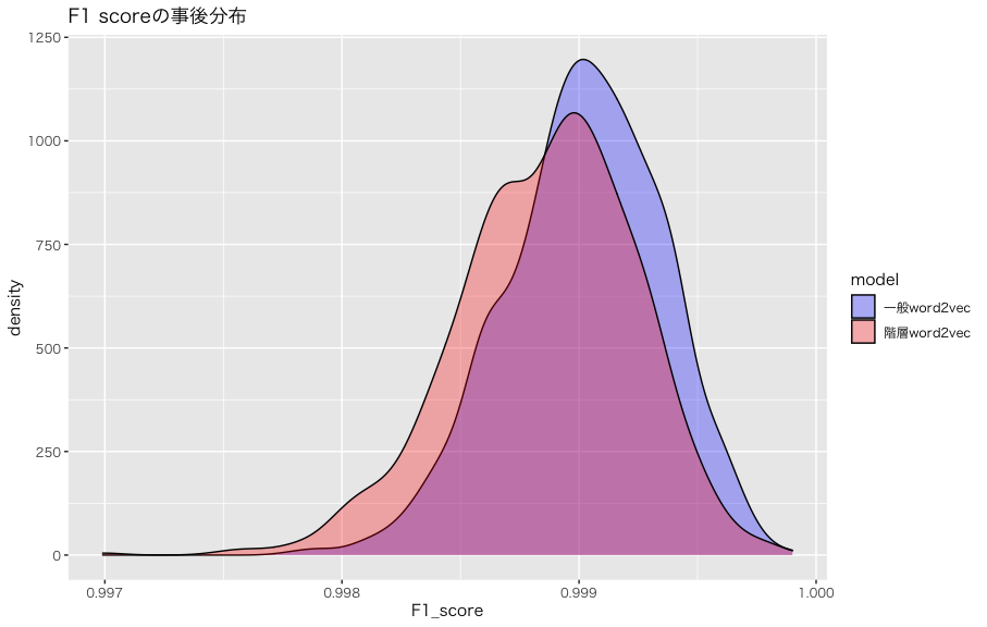
なんか完璧に近い精度が出ちゃったんだけどw
F1スコア0.999ってなんなんw
(データリークないのかな、、、)
階層ベイズword2vecのF1スコアの事後分布が全体的に低いところにありますが、両者に統計的に有意な差がなく、同じ精度であると判断しても問題ないと思います。
分散表現の違い
最後に、学習された分散表現を比較します。
まず、必要なパラメータを抽出して行列に整形してから、t-SNEで解析します。
word_embedding_bw2v <- m_bw2v_summary |>
  dplyr::filter(stringr::str_detect(variable, "word_embedding")) |>
  dplyr::pull(mean) |>
  matrix(ncol = 30)

category_embedding_hbw2v <- m_hbw2v_summary |>
  dplyr::filter(stringr::str_detect(variable, "category_embedding")) |>
  dplyr::pull(mean) |>
  matrix(ncol = 30)

word_embedding_hbw2v <- m_hbw2v_summary |>
  dplyr::filter(stringr::str_detect(variable, "word_embedding")) |>
  dplyr::pull(mean) |>
  matrix(ncol = 30)

set.seed(12345)
tsne_bw2v <- Rtsne::Rtsne(
  word_embedding_bw2v
)
tsne_hbw2v <- Rtsne::Rtsne(
  rbind(category_embedding_hbw2v, word_embedding_hbw2v)
)

g_bw2v <- item_category_master |>
  dplyr::bind_cols(
    x1 = tsne_bw2v$Y[,1],
    x2 = tsne_bw2v$Y[,2]
  ) |>
  ggplot2::ggplot() +
  ggplot2::geom_point(ggplot2::aes(x = x1, y = x2, color = category), alpha = 0.3) +
  ggplot2::xlab("dimension 1") +
  ggplot2::ylab("dimension 2") +
  ggplot2::ggtitle("Ordinary Bayesian word2vec\nVisualization by t-SNE")


g_hbw2v <- tibble::tibble(
  category = c(rep("parent_category", nrow(category_master)), item_category_master$category),
  category_code = c(category_master$category, item_category_master$category_code),
  x1 = tsne_hbw2v$Y[,1],
  x2 = tsne_hbw2v$Y[,2]
) |>
  ggplot2::ggplot() +
  ggplot2::geom_point(ggplot2::aes(x = x1, y = x2, color = category), alpha = 0.3) +
  ggplot2::xlab("dimension 1") +
  ggplot2::ylab("dimension 2") +
  ggplot2::ggtitle("Hierarchical Bayesian word2vec\nVisualization by t-SNE")
まず、階層のないベイズword2vecが学習した文案表現のt-SNEの結果を確認します:
g_bw2v
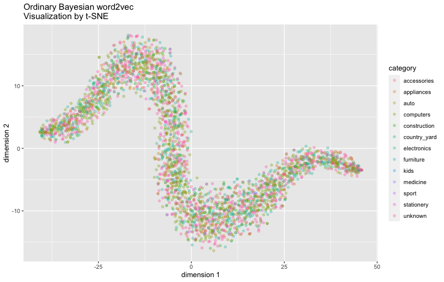
なんかヘビみたいな形ですね。
図の中の点が一つの商品を表し、カテゴリごとに色をつけました。
商品カテゴリによってクラスタになっておらず、全体が混ざっているところを特に協調したいです。
続いて階層ベイズword2vecも確認しましょう:
g_hbw2v
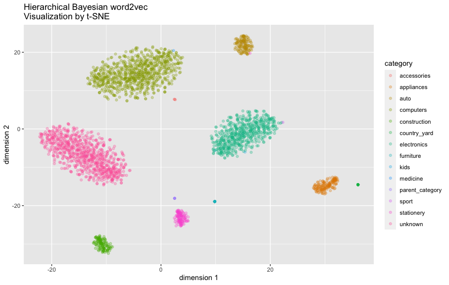
階層ベイズの場合、事前分布の設定通りに、カテゴリ別のクラスタが確認できます。また、商品の分散表現(word embedding)ごとに異なる分散パラメータを設定していますので、データに十分な証拠があれば、クラスタからの逸脱も許されます。実際複数の点がクラスタの中心から離れた場所に位置しています。
t-SNEの図からも分かるように、商品の分散表現同士の類似度を求めるとき、階層ベイズword2vecは基本的に同じカテゴリの商品にしか高い類似度を付与しないが、普通のベイズword2vecの場合はこのような保証がありません。
なので、例えば量販店部門の統括マネージャーからの、店舗でパソコンを購入したユーザーにはパソコンを中心に、文房具を購入したユーザーには文房具を中心にそれぞれレコメンドしてほしいという要望に対して、階層ベイズ版のword2vecを利用したソフトなルールベースの形で実現できます。
全くの余談ですが、私がもし家電量販店のデータサイエンティストでこのような要望を受けたら、まずユーザーがそもそも同じカテゴリの商品を求めているのかの仮説を検証するため、普通のベイズword2vecと階層ベイズword2vecをABテストで戦わせることを提案します。
検証データに対する本物フラグ分類というタスクにほぼ同一の精度を達成した二つのモデルが、レコメンドタスクで異なる性能(CVRの差)を出しそうで興味深いですね。
練習問題
さて、ここで練習問題です。興味ある方は回答してみてください。
-
商品の分散表現(word embedding)同士のコサイン類似度を計算する方法とその解釈方法を説明してください
-
ミクロ経済学の商品の補完財・代替財の定義を説明してください
-
商品の分散表現同士のコサイン類似度は、補完財・代替財を測る指標として適切ですか?三つの用語の定義を引用しながら説明してください
-
商品の分散表現同士のコサイン類似度は、補完財・代替財を測る指標として適切だと答えた場合、普通のベイズword2vecの方を利用しますか?それとも階層ベイズword2vecを利用しますか?用語の定義とモデルの定式化を引用しながら説明してください
-
商品の分散表現同士のコサイン類似度は、補完財・代替財を測る指標として適切だと答えた場合、hier_bayesian_word2vec.stanかbayesian_word2vec.stan
のgenerated quantitiesブロック内に、スルツキー行列(Slutsky matrix)をサンプリングするための処理を追加してください -
商品の分散表現同士のコサイン類似度は、補完財・代替財を測る指標として適切ではないと答えた場合、コサイン類似度と補完財・代替財の指標はそれぞれどのようなビジネスの意思決定で役に立つのか?本記事の背景の家電量販店のデータサイエンティストの立場で答えてください
-
商品の分散表現同士のコサイン類似度は、補完財・代替財を測る指標として適切ではないと答えた場合、補完財・代替財を測る指標を測るために必要なデータおよびその取得案とROIの試算を本記事の背景の家電量販店のデータサイエンティストの立場で答えてください。データ収集の投資に値しないと判断した場合は、その旨と理由を回答してください
参考文献
Blei, David M., Andrew Y. Ng, and Michael I. Jordan. "Latent dirichlet allocation." Journal of Machine Learning Research 3.Jan (2003): 993-1022.
Mikolov, Tomas, et al. "Distributed representations of words and phrases and their compositionality." Advances in neural information processing systems 26 (2013).
Rudolph, Maja, et al. "Exponential family embeddings." Advances in Neural Information Processing Systems 29 (2016).
呉 東文「分布族埋め込みで可視化するレコード・チャイナの言説」Working Paper No. 6(一橋大学社会科学高等研究院グローバル・ガバナンス研究センター, 2023)