住宅価格を予測する(データ前処理編：前半）ver1.1

はじめに

　Kaggleにてチュートリアルとして用いられるSale Price(住宅価格）予測問題について解いていきます。前回は一次回帰により簡単に予測しましたが、今回は欠損値保管、カテゴリー変数の変換、新しい特徴量の指定などのデータ前処理を行います。後半で機械学習及び予測を行っていきます。

後半
https://qiita.com/Fumio-eisan/items/7e13695ef5ccc6acf61c

こちらを全面的に参考にさせて頂きました。
https://www.kaggle.com/serigne/stacked-regressions-top-4-on-leaderboard

• python　3.7.4
• seaborn 0.10.0
• numpy 1.18.1
• pandas 0.25.3
• matplotlib 3.1.3
• scipy 1.4.1

データ前処理

　まずは下記URLからtrain,test.csvデータを任意フォルダにダウンロードします。
https://www.kaggle.com/c/house-prices-advanced-regression-techniques

必要なライブラリの読み込み

import numpy as np # linear algebra
import pandas as pd # data processing, CSV file I/O (e.g. pd.read_csv)
%matplotlib inline
import matplotlib.pyplot as plt  # Matlab-style plotting
import seaborn as sns
color = sns.color_palette()
sns.set_style('darkgrid')
import warnings
def ignore_warn(*args, **kwargs):
    pass
warnings.warn = ignore_warn #ignore annoying warning (from sklearn and seaborn)


from scipy import stats
from scipy.stats import norm, skew #for some statistics


pd.set_option('display.float_format', lambda x: '{:.3f}'.format(x)) #Limiting floats output to 3 decimal points

データ読み込み

train = pd.read_csv('train.csv')
test = pd.read_csv('test.csv')

今回は、最初にtrain,testデータを両方読み込みます。

Id列の削除

train_ID = train['Id']
test_ID = test['Id']

train.drop("Id", axis = 1, inplace = True)
test.drop("Id", axis = 1, inplace = True)

Id列は不必要なため削除し、別の変数として定義しておきます。

外れ値の削除

fig, ax = plt.subplots()
ax.scatter(x = train['GrLivArea'], y = train['SalePrice'])
plt.ylabel('SalePrice', fontsize=13)
plt.xlabel('GrLivArea', fontsize=13)
plt.show()

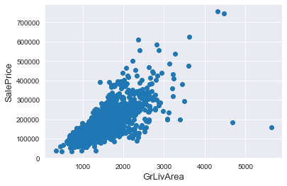
　GrLivAreaとSalePriceを見ると、GrLivAreaが4000以上かつSalePriceが300000未満のところに2つ外れているプロットがあります。これは予測するうえで当たらなくなる要因となるので、削除します。

#Deleting outliers
train = train.drop(train[(train['GrLivArea']>4000) & (train['SalePrice']<300000)].index)

#Check the graphic again
fig, ax = plt.subplots()
ax.scatter(train['GrLivArea'], train['SalePrice'])
plt.ylabel('SalePrice', fontsize=13)
plt.xlabel('GrLivArea', fontsize=13)
plt.show()

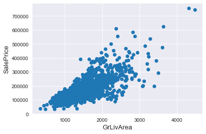
　削除することができました。ただ、この削除は安易に進めてはいけないと思います。その外れ値がデータとしてもつ意味を考慮したうえで行うことが望ましいと思います。

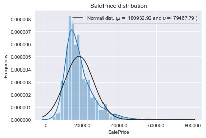
データの標準化

　続いて、SalePriceをlogを取り正規分布に乗るように処理をします。その詳しい理由については私自身、実感を持って説明できないところがありますので、別途まとめたいと思います。

https://qiita.com/ttskng/items/2a33c1ca925e4501e609
https://ishitonton.hatenablog.com/entry/2019/02/24/184253

#We use the numpy fuction log1p which  applies log(1+x) to all elements of the column
train["SalePrice"] = np.log1p(train["SalePrice"])

#Check the new distribution 
sns.distplot(train['SalePrice'] , fit=norm);

# Get the fitted parameters used by the function
(mu, sigma) = norm.fit(train['SalePrice'])
print( '\n mu = {:.2f} and sigma = {:.2f}\n'.format(mu, sigma))

#Now plot the distribution
plt.legend(['Normal dist. ($\mu=$ {:.2f} and $\sigma=$ {:.2f} )'.format(mu, sigma)],
            loc='best')
plt.ylabel('Frequency')
plt.title('SalePrice distribution')

#Get also the QQ-plot
fig = plt.figure()
res = stats.probplot(train['SalePrice'], plot=plt)
plt.show()

変更前

変更後

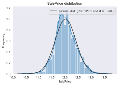
　対数を取ることにより正規分布化させることができました。

　特徴エンジニアリング(Feature Engineering)の実施

　欠損値の取り扱い、新しい特徴量の決定、カテゴリー変数のダミー変数化を行っていきます。
　まずはtrainデータとtestデータを合致させます。

ntrain = train.shape[0]
ntest = test.shape[0]
y_train = train.SalePrice.values
all_data = pd.concat((train, test)).reset_index(drop=True)
all_data.drop(['SalePrice'], axis=1, inplace=True)
print("all_data size is : {}".format(all_data.shape))

欠損値取り扱い

　次に欠損値を処理していきます。

all_data["PoolQC"] = all_data["PoolQC"].fillna("None")
all_data["MiscFeature"] = all_data["MiscFeature"].fillna("None")
all_data["Alley"] = all_data["Alley"].fillna("None")
all_data["Fence"] = all_data["Fence"].fillna("None")
all_data["FireplaceQu"] = all_data["FireplaceQu"].fillna("None")
all_data["LotFrontage"] = all_data.groupby("Neighborhood")["LotFrontage"].transform(
    lambda x: x.fillna(x.median()))
for col in ('GarageType', 'GarageFinish', 'GarageQual', 'GarageCond'):
    all_data[col] = all_data[col].fillna('None')

for col in ('BsmtFinSF1', 'BsmtFinSF2', 'BsmtUnfSF','TotalBsmtSF', 'BsmtFullBath', 'BsmtHalfBath'):
    all_data[col] = all_data[col].fillna(0)
for col in ('BsmtQual', 'BsmtCond', 'BsmtExposure', 'BsmtFinType1', 'BsmtFinType2'):
    all_data[col] = all_data[col].fillna('None')
all_data["MasVnrType"] = all_data["MasVnrType"].fillna("None")
all_data["MasVnrArea"] = all_data["MasVnrArea"].fillna(0)
all_data['MSZoning'] = all_data['MSZoning'].fillna(all_data['MSZoning'].mode()[0])
all_data = all_data.drop(['Utilities'], axis=1)
all_data["Functional"] = all_data["Functional"].fillna("Typ")
all_data['Electrical'] = all_data['Electrical'].fillna(all_data['Electrical'].mode()[0])
all_data['KitchenQual'] = all_data['KitchenQual'].fillna(all_data['KitchenQual'].mode()[0])
all_data['Exterior1st'] = all_data['Exterior1st'].fillna(all_data['Exterior1st'].mode()[0])
all_data['Exterior2nd'] = all_data['Exterior2nd'].fillna(all_data['Exterior2nd'].mode()[0])
all_data['SaleType'] = all_data['SaleType'].fillna(all_data['SaleType'].mode()[0])
all_data['MSSubClass'] = all_data['MSSubClass'].fillna("None")

カテゴリー変数のダミー変数化

　次にカテゴリー変数をダミー変数化します。
　この操作を行う上での注意点として、訓練用データとテスト用データは最初に合致させたデータを作りましょう。そして、その合致データを処理していきましょう。別々のデータとしてダミー変数処理を行うと、列数が一致しないことが発生するため、最後に予測させることができなくなります。

　私は別々に処理して、後で列数が合わないことがありました。無理に列数を揃えようとダミー変数で足りないもの、多いものをcsvに出力させて地道に見ましたが諦めました。。初めから合致させましょう。。

all_data = pd.get_dummies(all_data)
print(all_data.shape)

まとめ

　今回は以上になります。後半では実際に解析を行いモデルの高精度化を狙っていきます。

後半
https://qiita.com/Fumio-eisan/items/7e13695ef5ccc6acf61c

プログラム全文はこちらです。
https://github.com/Fumio-eisan/houseprice20200301