imbalanced-learnパッケージのRandomUnderSampler関数でアンダーサンプリングの方法です。注意点を含めていくつか書いておきます。imbalanced-learnには他のアンダーサンプリングやオーバーサンプリング、両者を同時に行う関数など様々あります。まずは入門としてRandomUnderSampler関数を使いました。
関連トピックとして以下の記事があります。

環境

Python3.7.13でGoogle Colaboratory上で動かしています。Google Colabプリインストールされているパッケージはそのまま使っています。

Package	Version	備考
imblearn	0.9.1	Google Colabプリインストール
matplotlib	3.2.2	Google Colabプリインストール
numpy	1.21.6	Google Colabプリインストール
pandas	1.3.5	Google Colabプリインストール
scikit-learn	1.0.2	Google Colabプリインストール

プログラム

1. Import

パッケージインポート。

from imblearn.under_sampling import RandomUnderSampler
import pandas as pd
import matplotlib.pyplot as plt
from matplotlib.ticker import PercentFormatter
import numpy as np
from sklearn.datasets import make_classification
from sklearn.linear_model import LogisticRegression
from sklearn.metrics import ConfusionMatrixDisplay, log_loss
from sklearn.model_selection import train_test_split

2. 不均衡データ作成

make_classification関数を使って正例が１％の不均衡データを生成し、訓練と評価データに分割。

def make_df():
    X, y = make_classification(n_samples=10_000, weights=[0.99, 0.01])
    X_train, X_test, y_train, y_test = train_test_split(X, y, train_size=0.9)
    return X_train, X_test, y_train, y_test

X_train, X_test, y_train, y_test = make_df()

3. 訓練と評価実施

RandomUnderSampler関数を使ってアンダーサンプリングします。注意点としては、sampling_strategyに渡すパラメータは以下の値です。

\frac{アンダーサンプリング後負例数}{アンダーサンプリング前負例数}

上記のように割合を渡す以外の方法もあるようですが、詳しくは公式文書を参照ください。
アンダーサンプリング率を変更し、以下の流れで実施。

アンダーサンプリング実施
ロジスティック回帰で訓練
評価データで予測し、対数ロスを計算
予測確率のCalibration実施
Calibration後の予測確率で対数ロス計算

results = []
train_count = np.unique(y_train, return_counts=True)
lfunc = lambda x: x/(x+((1-x)/beta))

for i in range(1, 21):
    # サンプリング後の負例数/ サンプリング前の負例数
    beta = 1 / i

    # 正例数 / (DS前 負例数 * サンプリング率)
    ratio = train_count[1][1] / ( train_count[1][0] * beta)
    X_sampled, y_sampled = RandomUnderSampler(sampling_strategy=ratio).fit_resample(X_train, y_train)
    sample_count = np.unique(y_sampled, return_counts=True)

    # 訓練および推論
    clf = LogisticRegression()
    clf.fit(X_sampled, y_sampled)
    y_pred_proba = clf.predict_proba(X_test)
    lloss_non_calib = log_loss(y_test, y_pred_proba[:,1])

    # Calibration
    calibrated = lfunc(y_pred_proba[:,1])
    lloss_calib = log_loss(y_test, calibrated)
    results.append([i, sample_count[1][0], beta, lloss_non_calib, lloss_calib])

# 最終行のみヒストグラム表示
else:
    plt.hist(calibrated)

参考に最終行(サンプリング率が0.05)の予測確率ヒストグラムです。Calibrationによって自信過剰を抑えられるのですが、予測確率が0.1以下と低く集中します。詳しいシミュレーションは別記事「不均衡データへのダウンサンプリング後のCalibration」に書きました。

4. 対数ロスグラフ表示

対数ロスをグラフに表示してみます。

df_result = pd.DataFrame(results, columns=['i', 'sample num', 'BETA', 'lloss', 'lloss calibrated'])
df_result.index = round(df_result['BETA'], 3)

_, axes = plt.subplots(nrows=2, figsize=(10, 7), constrained_layout=True)
df_result.loc[:,['lloss', 'lloss calibrated']].plot.bar(ax=axes[0])
axes[0].grid(axis='y', linestyle='dotted')
axes[0].axhline(y=results[0][3], ls='--', color='red', alpha=0.6)

df_result['relative'] = df_result.loc[:,['lloss calibrated']] / results[0][3]
df_result.loc[:,['relative']].plot.bar(ax=axes[1])
axes[1].grid(axis='y', linestyle='dotted')
axes[1].set_ylim([0.9, 1.1])
axes[1].yaxis.set_major_formatter(PercentFormatter(1.0))
axes[1].axhline(y=1, ls='--', color='red', alpha=0.6)

plt.show()

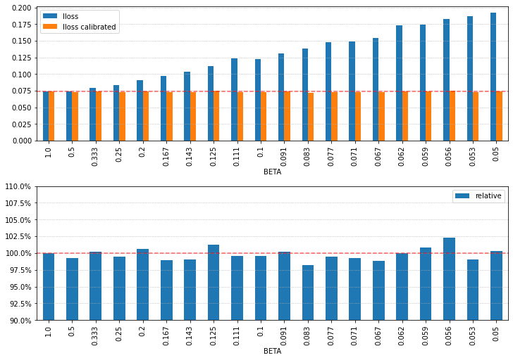
上のグラフがCalibration前後の対数ロスで、Y軸の赤点線はアンダーサンプリング未実施時の対数ロスの値です。
下のグラフはCalibration後の対数ロスの値を相対表示(100%はアンダーサンプリング未実施時で赤点線で強調)。
アンダーサンプリングによって対数ロスが低下する、みたいな結果だとわかりやすいのですが、そんなこともなかったです。正直、どういう場合に効果があるのかわからないですが、Facebookの例のように効果がある場合もあります。私が仕事で効果があったこともありました。

imbalanced-learnのRandomUnderSamplerでアンダーサンプリング

環境

プログラム

1. Import

2. 不均衡データ作成

3. 訓練と評価実施

4. 対数ロスグラフ表示