BERTを勉強していてseq2seqのAttentionについて整理しました。モデル部分は理解しましたが、訓練ジョブを流す部分などはほとんど見ていないですし解説もしていません。seq2seqについては記事「【Keras入門(7)】単純なSeq2Seqモデル定義」で以前解説をしました。
もともとは以下のオンライン講座を受講していて、Attentionに関する理解を深めようとしたのがきっかけでした。
以下のTensorFlowのチュートリアルを使って学習しました。
チュートリアルに以下の記載があるとおり、少し古い考えですが Attention を理解する上で重要だと信じ時間をかけました。
While this architecture is somewhat outdated it is still a very useful project to work through to get a deeper understanding of attention mechanisms (before going on to Transformers).
理解にあたり以下を参考にしました。私がPyTorchを使っていないことには、深い理由はないです。
モデル解説
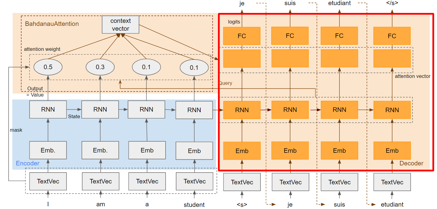
モデル全体
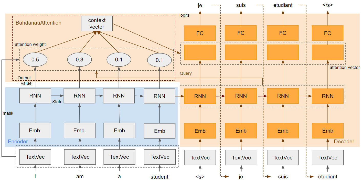
モデル詳細
Text Processing

テキストをTokenizeとID化しています(正確には以下の処理)。
- ユニコード正規化
- 大文字の小文字化
- テキストのTokenize
- [START]と[END]を先頭と末尾に追加
- Tokenに対して辞書を使ったID化
出力のShapeに「最大Token数」とありますが、[START]と[END]が加わっていることが注意点です。「BS」はBatch Sizeを意味します。
| 入出力 | Shape | 例 |
|---|---|---|
| 入力 | BS * 1 | [['I like you'],['This is a pen']] |
| 出力 | BS * 最大Token数 | [[5 4 3 2 6 0],[5 1 1 1 1 6]] |
TextVectorization関数を使っています。確か日本語はTokenizeできないので、MeCabなどを使わないといけなかったはず。
max_vocab_size = 5000

# Encoder
input_text_processor = tf.keras.layers.TextVectorization(
    standardize=tf_lower_and_split_punct,
    max_tokens=max_vocab_size)

# Decoder
output_text_processor = tf.keras.layers.TextVectorization(
    standardize=tf_lower_and_split_punct,
    max_tokens=max_vocab_size)
パラメータstandardizeに渡した関数tf_lower_and_split_punctでユニコード正規化・小文字化などをしています。
ユニコード正規化では「㍍」を「メートル」に変換などをしています。軽くしか試していないのでtf_text.normalize_utf8が日本語処理として実用に耐えうるレベルか不明。
def tf_lower_and_split_punct(text):
  # Split accecented characters.
  text = tf_text.normalize_utf8(text, 'NFKD')
  text = tf.strings.lower(text)
  # Keep space, a to z, and select punctuation.
  text = tf.strings.regex_replace(text, '[^ a-z.?!,¿]', '')
  # Add spaces around punctuation.
  text = tf.strings.regex_replace(text, '[.?!,¿]', r' \0 ')
  # Strip whitespace.
  text = tf.strings.strip(text)

  text = tf.strings.join(['[START]', text, '[END]'], separator=' ')
  return text
Encoder
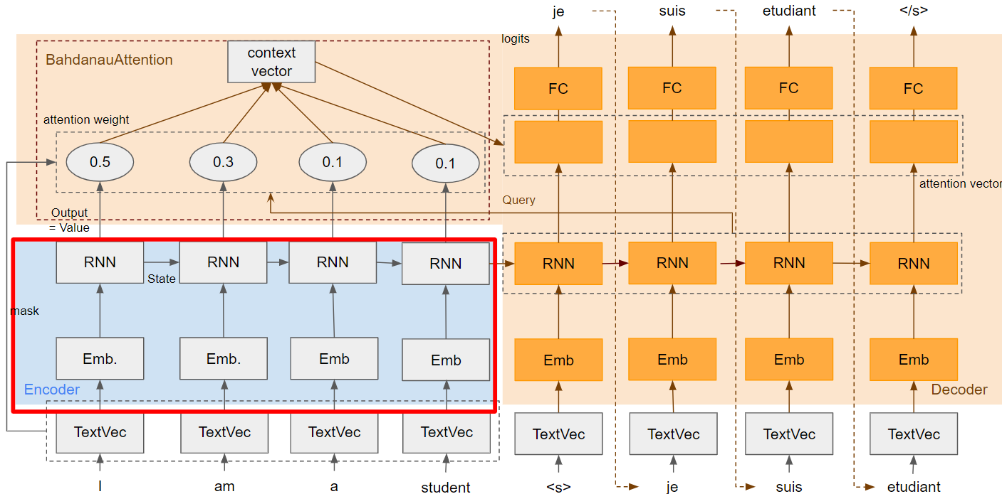
Attention固有の内容は特になく通常のEncorderです。RNNセルにはGRUを使っています。
| 入出力 | Shape |
|---|---|
| Embedding入力 | BS * 最大Token数 |
| Embedding->RNN | BS * 最大Token数 * Embedding Unit数 |
| RNN出力(State) | BS * RNN Unit数 |
| RNN出力(Output) | BS * 最大Token数 * RNN Unit数 |
class Encoder(tf.keras.layers.Layer):
  def __init__(self, input_vocab_size, embedding_dim, enc_units):
    super(Encoder, self).__init__()
    self.enc_units = enc_units
    self.input_vocab_size = input_vocab_size

    # The embedding layer converts tokens to vectors
    self.embedding = tf.keras.layers.Embedding(self.input_vocab_size,
                                               embedding_dim)

    # The GRU RNN layer processes those vectors sequentially.
    self.gru = tf.keras.layers.GRU(self.enc_units,
                                   # Return the sequence and state
                                   return_sequences=True,
                                   return_state=True,
                                   recurrent_initializer='glorot_uniform')

  def call(self, tokens, state=None):
    # 2. The embedding layer looks up the embedding for each token.
    vectors = self.embedding(tokens)

    # 3. The GRU processes the embedding sequence.
    #    output shape: (batch, s, enc_units)
    #    state shape: (batch, enc_units)
    output, state = self.gru(vectors, initial_state=state)

    # 4. Returns the new sequence and its state.
    return output, state
Decoder
Decoderの全体部分は後回しにして、Attentionから説明します。
Attention
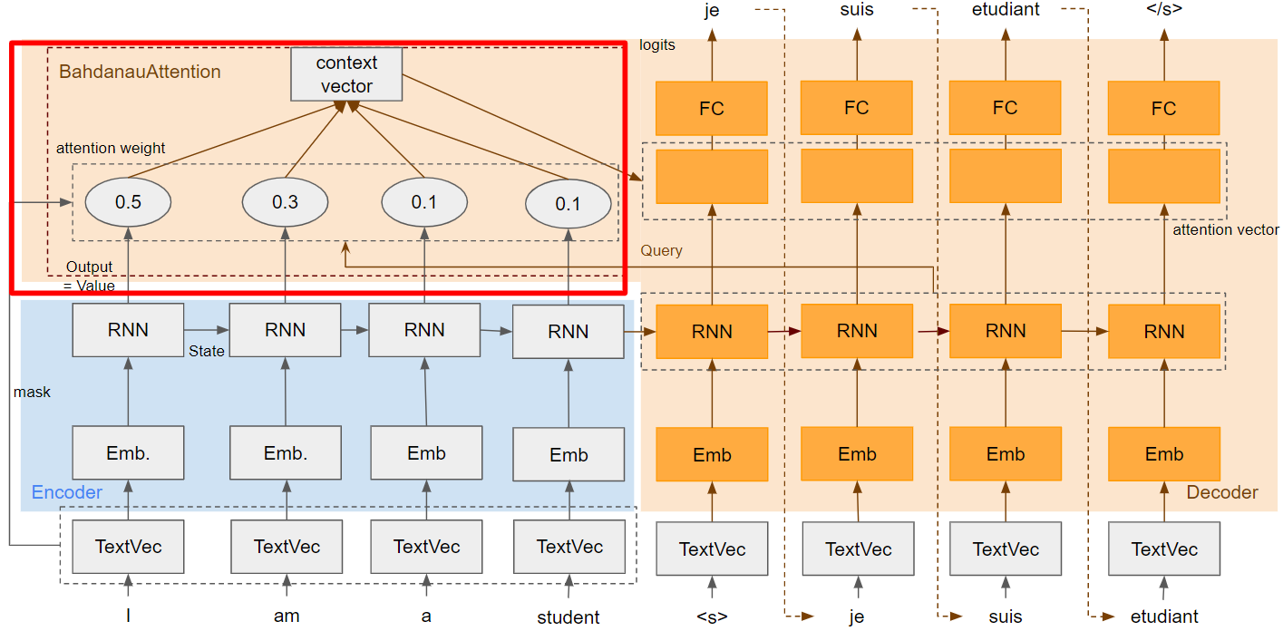
このレイヤが今回の本題です。
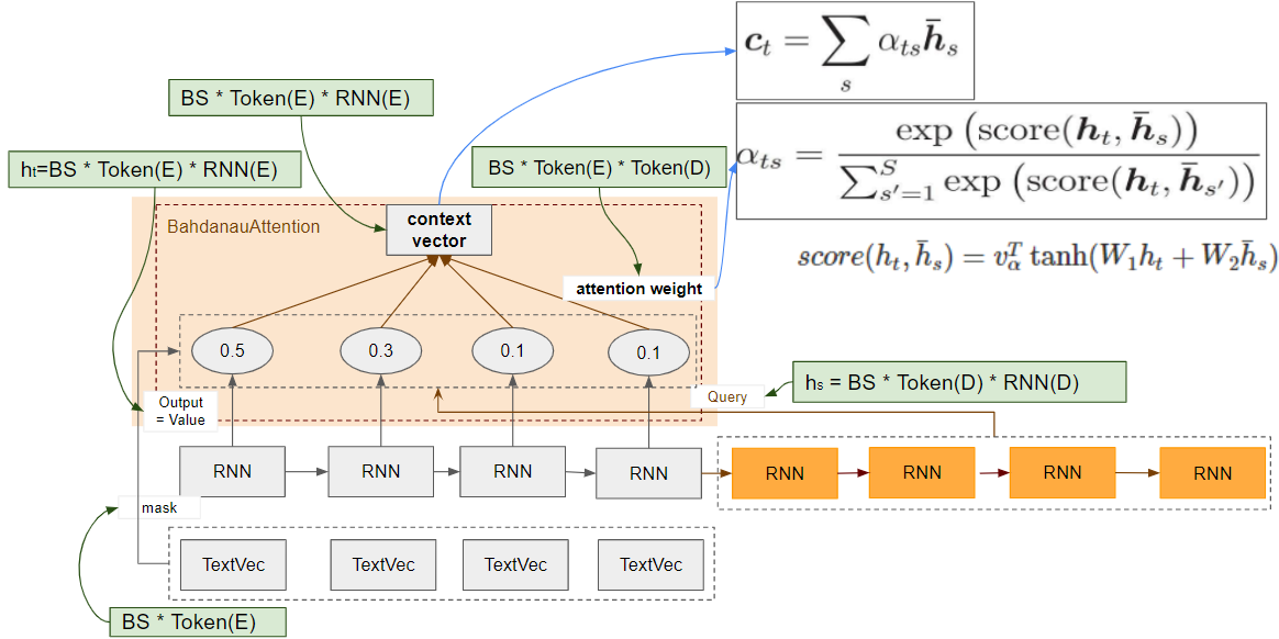
少し複雑なので関連部分をクローズアップして計算式とShapeを追記しました。Shapeの(E)はEncoder、(D)はDecoderを示しています(Token(D): DecoderのToken数)。添字のsはEncoderのindex、tはDecoderのindexです。
| 入出力 | Shape |
|---|---|
| Value Mask: TextVectorization出力->Attention入力 | BS * Token数(E) |
| Value: RNN出力(Output)->Attention入力 | BS * Token数(E) * RNN Unit数(E) |
| Query: RNN出力(Output)->Attention入力 | BS * Token数(D) * RNN Unit数(D) |
| Attention weight: Attention出力 | BS * Token数(E) * Token数(D) |
| Context Vector: Attention出力 | BS * Token数(E) * RNN Unit数(E) |
Attention weight
score部分の計算にBahdanau's additive attentionを使っています。今回は使いませんが、もう一つ有名なLuong's multiplicative style というのもあるようです。
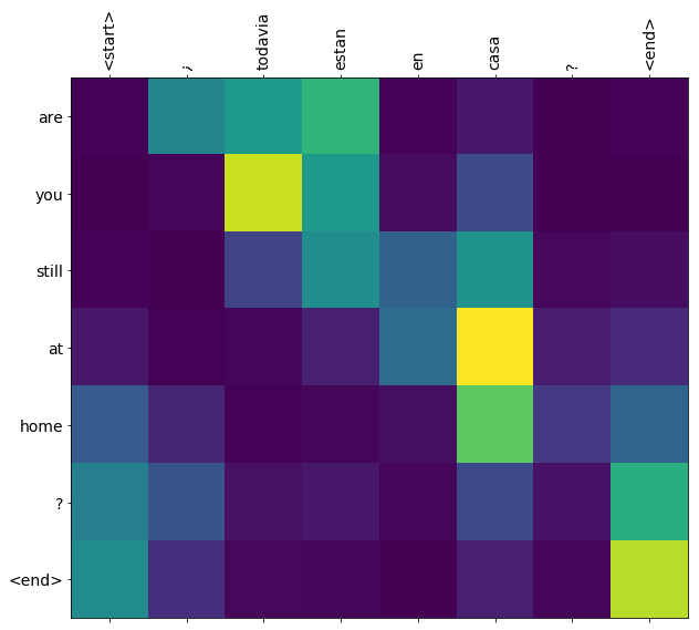
Attention weightはチュートリアルのトップにあるように、EncoderのTokenとDecoderのTokenのマトリックスです(バッチサイズは除く)。どのDecoderのTokenからAttentionされているのがどのEncoderのTokenの割合です(合計が1の確率変数)。Attention weightのshapeは「BS * Token数(E) * Token数(D)」になります。
Attention weightの計算式です。tanhは活性化関数です。score部の$v_{\alpha}^T$は学習パラメータなのが注意点です。
\alpha_{ts} = \frac{\exp(score(h_t, \bar{h}_s))}{\sum_{s'=1}^{S} \exp(score(h_t, \bar{h}_{s'}))}\\
score(h_t, \bar{h}_s)=v_{\alpha}^T \tanh (W_1 h_t + W_2 \bar{h}_s)
Attention weightは、$score(h_t, \bar{h}_s)$のsoftmax関数になっています。参考に下記がsoftmax関数。
{y_i = \frac{\exp(x_i)}{\sum_{j=1}^N \exp(x_j)}}
内部的にはvalueもkeyもmaskをtf.keras.layers.AdditiveAttentionに渡しています。maskをどう使っているか細かくは調べていません(単純に計算から除外していると推測しています)。
class BahdanauAttention(tf.keras.layers.Layer):
  def __init__(self, units):
    super().__init__()
    # For Eqn. (4), the  Bahdanau attention
    self.W1 = tf.keras.layers.Dense(units, use_bias=False)
    self.W2 = tf.keras.layers.Dense(units, use_bias=False)

    self.attention = tf.keras.layers.AdditiveAttention()

  def call(self, query, value, mask):
    # From Eqn. (4), `W1@ht`.
    w1_query = self.W1(query)

    # From Eqn. (4), `W2@hs`.
    # from memory to key
    w2_key = self.W2(value)

    # 3つ目の次元(RNN の unit)をなくしてすべてTrueのBool型
    query_mask = tf.ones(tf.shape(query)[:-1], dtype=bool)
    value_mask = mask

    context_vector, attention_weights = self.attention(
        inputs = [w1_query, value, w2_key],
        mask=[query_mask, value_mask],
        return_attention_scores = True,
    )

    return context_vector, attention_weights
maskはこんな中身。boolで、Tokenがpaddingされている部分はFalse。
tf.Tensor(
[[ True  True  True ... False False False]
 ...
 [ True  True  True ... False False False]], shape=(128, 32), dtype=bool)
Context vector
Context vectorはAttention weightとDecoderのRNN Outputの内積の総和。
| 入出力 | Shape |
|---|---|
| Query: RNN出力(Output)->Context Vecotr入力 | BS * Token数(D) * RNN Unit数(D) |
| Attention weight: Context Vector入力 | BS * Token数(E) * Token数(D) |
| Context Vector: Attention出力 | BS * Token数(E) * RNN Unit数(E) |
計算式。
c_t = \sum_s \alpha_{ts} \bar{h}_s
コードは、「Attention weight」部分と共通。
Decoder 全体
最後にDecoder全体です。
| 入出力 | Shape |
|---|---|
| Embedding入力 | BS * 最大Token数 |
| Embedding->RNN | BS * 最大Token数 * Embedding Unit数 |
| RNN出力(State) | BS * RNN Unit数 |
| RNN出力(Output)->Attention Vecotr | BS * 最大Token数 * RNN Unit数 |
| Context Vector->Attention Vector | BS * 最大Token数 * RNN Unit数 |
| Attention Vector->Fully Connected | BS * 最大Token数 * RNN Unit数 |
| Fully Connected->Output | BS * 最大Token数 * 最大Vocabrary数 |
class Decoder(tf.keras.layers.Layer):
  def __init__(self, output_vocab_size, embedding_dim, dec_units):
    super(Decoder, self).__init__()
    self.dec_units = dec_units
    self.output_vocab_size = output_vocab_size
    self.embedding_dim = embedding_dim

    # For Step 1. The embedding layer convets token IDs to vectors
    self.embedding = tf.keras.layers.Embedding(self.output_vocab_size,
                                               embedding_dim)

    # For Step 2. The RNN keeps track of what's been generated so far.
    self.gru = tf.keras.layers.GRU(self.dec_units,
                                   return_sequences=True,
                                   return_state=True,
                                   recurrent_initializer='glorot_uniform')

    # For step 3. The RNN output will be the query for the attention layer.
    self.attention = BahdanauAttention(self.dec_units)

    # For step 4. Eqn. (3): converting `ct` to `at`
    self.Wc = tf.keras.layers.Dense(dec_units, activation=tf.math.tanh,
                                    use_bias=False)

    # For step 5. This fully connected layer produces the logits for each
    # output token.
    self.fc = tf.keras.layers.Dense(self.output_vocab_size)
def call(self,
         inputs: DecoderInput,
         state=None) -> Tuple[DecoderOutput, tf.Tensor]:

  # Step 1. Lookup the embeddings
  vectors = self.embedding(inputs.new_tokens)

  # Step 2. Process one step with the RNN
  rnn_output, state = self.gru(vectors, initial_state=state)

  # Step 3. Use the RNN output as the query for the attention over the
  # encoder output.
  context_vector, attention_weights = self.attention(
      query=rnn_output, value=inputs.enc_output, mask=inputs.mask)

  # Step 4. Eqn. (3): Join the context_vector and rnn_output
  #     [ct; ht] shape: (batch t, value_units + query_units)
  context_and_rnn_output = tf.concat([context_vector, rnn_output], axis=-1)

  # Step 4. Eqn. (3): `at = tanh(Wc@[ct; ht])`
  attention_vector = self.Wc(context_and_rnn_output)

  # Step 5. Generate logit predictions:
  logits = self.fc(attention_vector)

  return DecoderOutput(logits, attention_weights), state
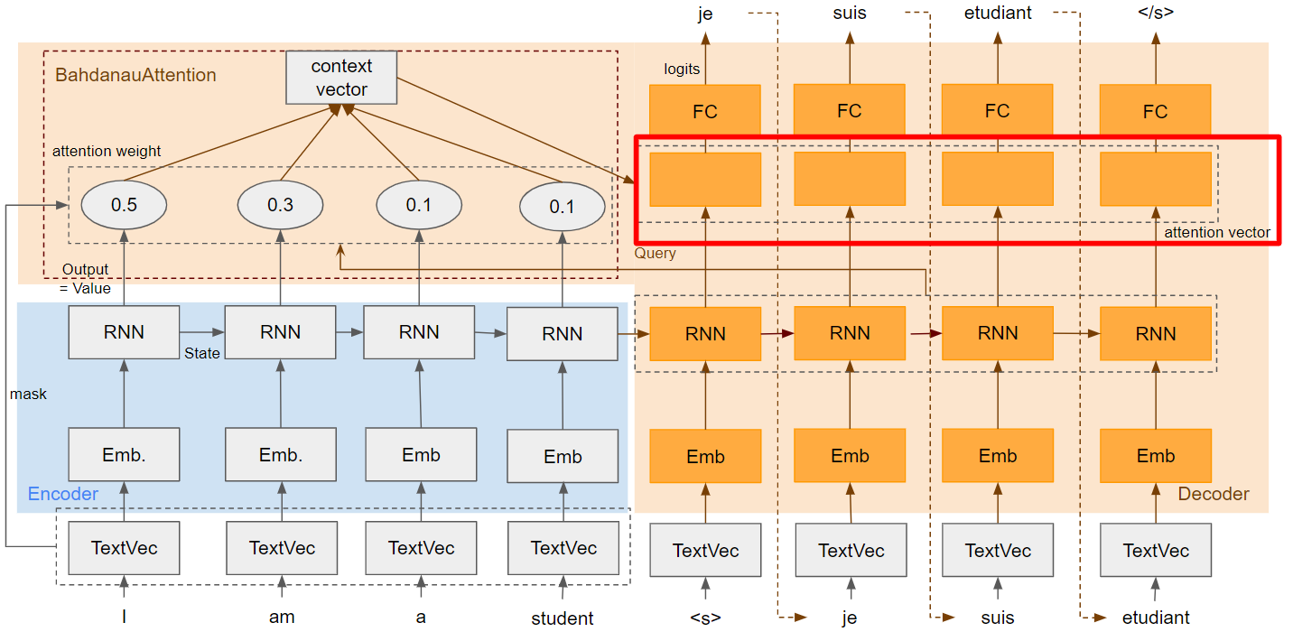
Attention Vector
Attention Vecotor部分の補足。Decoderの一部です。
計算式です。
\alpha_t = f(c_t,h_t) = \tanh (W_c[c_t;h_t])
Decoder RNNのoutputと Context Vectorを結合して、密結合層に入力しているのがわかります。
# Step 4. Eqn. (3): Join the context_vector and rnn_output
  #     [ct; ht] shape: (batch t, value_units + query_units)
  context_and_rnn_output = tf.concat([context_vector, rnn_output], axis=-1)

  # Step 4. Eqn. (3): `at = tanh(Wc@[ct; ht])`
  # self.Wcの活性化関数がtanhにしている
  attention_vector = self.Wc(context_and_rnn_output)
少しだけメモありプログラムGitHubリンク
TensorFlow公式チュートリアル「Neural machine translation with attention」をコピーし、メモしたものをnmt_with_attention.ipynbとしてGitHubに置きました。大したことをメモしてないですが、ないよりマシレベル。