入門者に向けてKerasを使ったSeq2Seqを解説します。Seq2Seqは機械翻訳やチャットボットなどに使われます。
Google Colaboratoryを使っているのでローカルでの環境構築すらしていません。Google Colaboratoryについては「Google Colaboratory概要と使用手順(TensorFlowもGPUも使える)」の記事を参照ください。
以下のシリーズにしています。
- 【 Keras入門(1)】単純なディープラーニングモデル定義
- 【Keras入門(2)】訓練モデル保存(KerasモデルとSavedModel)
- 【Keras入門(3)】TensorBoardで見える化
- 【Keras入門(4)】Kerasの評価関数(Metrics)
- 【Keras入門(5)】単純なRNNモデル定義
- 【Keras入門(6)】単純なRNNモデル定義(最終出力のみ使用)
- 【Keras入門(7)】単純なSeq2Seqモデル定義 -> 本記事
使ったPythonパッケージ
Google Colaboratoryでインストール済の以下のパッケージとバージョンを使っています。KerasはTensorFlowに統合されているものを使っているので、ピュアなKerasは使っていません。Pythonは3.6です。
- tensorflow: 1.14.0
- Numpy: 1.16.5
- matplotlib: 3.0.3
処理概要
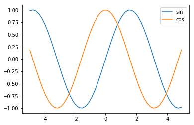
時系列データ予測として、正弦(sin)関数の値から余弦(cos)関数の値を予測します。
正弦(sin)関数と余弦(cos)関数は、こんなウネウネした値が変わっていく周期関数です。
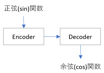
目的変数として正弦(sin)関数の値を10個渡して、余弦(cos)関数の値を10個返すようにします。
Seq2SeqはEncoder Decoderモデルとも呼ばれ、大雑把にはこんなデータパイプラインとなります。
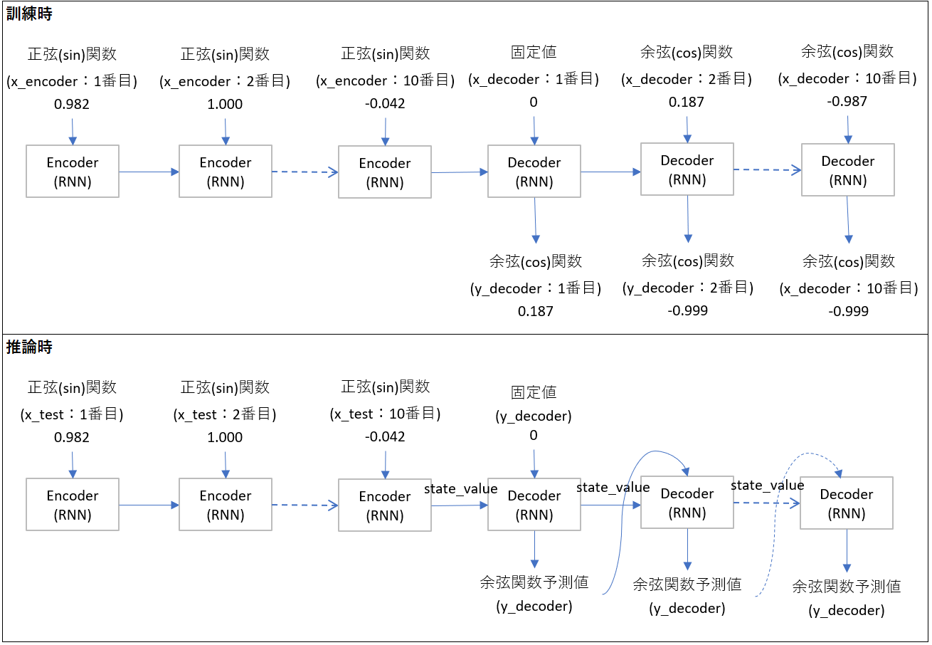
詳しく書くと、訓練と推論で以下のパイプラインです。後述するプログラムの変数名も書いています。
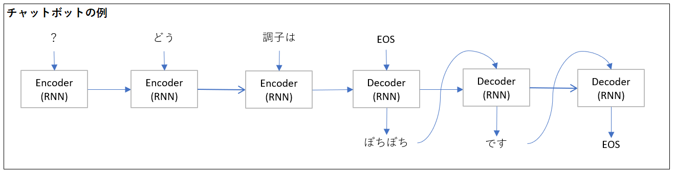
数値だとわかりにくいので、チャットボットを例にSeq2Seqを考えると下図のようになります。Encoderに入力するテキストは今回とは逆順になっているのが注意点です。
処理プログラム
プログラム全体はGitHubを参照ください。
1. ライブラリインポート
今回はmatplotlibとnumpyとtensorflowに統合されているkerasを使います。ピュアなkerasでも問題なく、インポート元を変えるだけです。
%matplotlib inline

import numpy as np
import matplotlib.pyplot as plt
from tensorflow.keras.models import Model
from tensorflow.keras.layers import Dense, LSTM, Input
from tensorflow.python.keras.utils.vis_utils import plot_model
2. 前処理
2.1. 正弦関数と余弦関数配列作成
-4.9から4.9までの50要素の等差数列(0.2間隔)の配列(axis_x)を作成し、対応する正弦関数の値の配列(sin_data)と余弦関数の値の配列(cos_data)を作成します。
axis_x = np.linspace(-4.9, 4.9) #-4.9から4.9までの50要素の等差数列作成

sin_data = np.sin(axis_x)  # 正弦(sin)関数
cos_data = np.cos(axis_x)  # 余弦(cos)関数
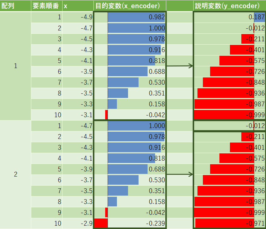
2.2. 説明変数(x_encoderとx_decoder)、目的変数(y_decoder)作成
Seq2Seqに流すための形に変換します。
エンコーダー入力(x_encoder)とデコーダー入力(x_decoder)、デコーダー出力(y_decoder)の配列を作成します。
N_RNN = 10  # 1セットのデータ数
N_SAMPLE = len(axis_x)-N_RNN  # サンプル数(今回は50-10=40)
N_IN_OUT = 1 # 入力層・出力層のニューロン数
N_MID = 20  # 中間層のニューロン数
shape_ = (N_SAMPLE, N_RNN, )

x_encoder = np.zeros(shape_)  # encoderの入力
x_decoder = np.zeros(shape_)  # decoderの入力
y_decoder = np.zeros(shape_)  # decoderの正解

for i in range(N_SAMPLE):
    x_encoder[i] = sin_data[i:i+N_RNN] #正弦(sin)関数を10づつ入力
    x_decoder[i, 1:] = cos_data[i:i+N_RNN-1]  # 最初の値は0のままでひとつ後にずらす
    y_decoder[i] = cos_data[i:i+N_RNN]  # 正解は余弦(cos)関数の値をそのまま入れる

# サンプル数、時系列の数、入力層のニューロン数にreshape
x_encoder = x_encoder.reshape(shape_+(N_IN_OUT,))
x_decoder = x_decoder.reshape(shape_+(N_IN_OUT,))
y_decoder = y_decoder.reshape(shape_+(N_IN_OUT,))
3. 訓練モデル定義
今回はSeq2SeqのRNNセルにLSTMを使用。
Seq2Seqは訓練と推論でモデル定義が異なるのがわかりにくいです。異なる理由は、先程の図で言うx_decoderにあります。訓練時はx_decoderに値を渡してあげますが、推論時はRNNの出力をそのまま使うため、両者のモデルが異なります。
訓練時の層を推論時に再利用します。どのオブジェクトを再利用しているかを明確にするため関数train_modelにして戻り値を定義しました。
def train_model():
    # input
    encoder_input = Input(shape=(N_RNN, N_IN_OUT)) # encoderの入力層
    decoder_input = Input(shape=(N_RNN, N_IN_OUT)) # decoderの入力層

    # encoder
    # return_stateをTrueにすることで、状態(htとメモリセル)が得られる。return_sequnceは不要
    encoder_output, state_h, state_c = LSTM(N_MID, return_state=True)(encoder_input)  # encoder LSTMの最終出力、状態(ht)、状態(メモリセル)
    encoder_states = [state_h, state_c] # LSTM結果のencoder_stateをdecoderのLSTM中間状態に渡す

    # decoder
    decoder_lstm = LSTM(N_MID, return_sequences=True, return_state=True)  # return_stateをTrueにすることで、状態(htとメモリセル)が得られる。
    decoder_output, _, _ = decoder_lstm(decoder_input, initial_state=encoder_states)  # encoderから得る状態を使用。状態(htとメモリセル)は不要
    decoder_dense = Dense(N_IN_OUT, activation='linear') # 予測で再利用のために全結合を定義
    decoder_output = decoder_dense(decoder_output)

    model = Model([encoder_input, decoder_input], decoder_output)  # 入力と出力を設定し、Modelクラスでモデルを作成
    model.compile(loss="mean_squared_error", optimizer="adam")
    model.summary()

    return model, encoder_input, encoder_states, decoder_lstm, decoder_dense
関数を呼び出し、出力してみます。
# 訓練モデル定義と出力
model, encoder_input, encoder_states, decoder_lstm, decoder_dense = train_model()
plot_model(model, show_shapes=True, show_layer_names=False)
summary関数で出てくる情報はこれ。
__________________________________________________________________________________________________
Layer (type)                    Output Shape         Param #     Connected to
==================================================================================================
input_1 (InputLayer)            [(None, 10, 1)]      0
__________________________________________________________________________________________________
input_2 (InputLayer)            [(None, 10, 1)]      0
__________________________________________________________________________________________________
lstm (LSTM)                     [(None, 20), (None,  1760        input_1[0][0]
__________________________________________________________________________________________________
lstm_1 (LSTM)                   [(None, 10, 20), (No 1760        input_2[0][0]
                                                                 lstm[0][1]
                                                                 lstm[0][2]
__________________________________________________________________________________________________
dense (Dense)                   (None, 10, 1)        21          lstm_1[0][0]
==================================================================================================
Total params: 3,541
Trainable params: 3,541
Non-trainable params: 0
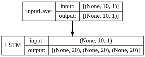
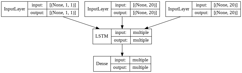
画像化するとこんなです。
4. 訓練
訓練実行です。だいたいLossが0.002くらいまで行きます。
最初はbatch_sizeをデフォルトの32で実行したのですが、データ数が少ないので、精度が40エポックでは良くなりませんでした。
history = model.fit([x_encoder, x_decoder], y_decoder, batch_size=8, epochs=40)

loss = history.history['loss']
plt.plot(np.arange(len(loss)), loss)
plt.show()

5. 予測モデル定義
予測モデルには訓練モデルで定義した層を再利用します。再利用箇所をわかりやすくするため関数化しています。
encoderとdecoderでモデルを分けているのが特徴的です。
def predict_model(encoder_input, encoder_states, decoder_lstm, decoder_dense):
    # encoderのモデルを構築
    encoder_model = Model(encoder_input, encoder_states)

    # decoderのモデルを構築
    decoder_input = Input(shape=(1, N_IN_OUT)) # (1, 1)

    # n_midは中間層のニューロン数(今回は20)
    # 状態(ht)と状態(メモリセル)の入力定義
    decoder_state_in = [Input(shape=(N_MID,)), Input(shape=(N_MID,))]

    decoder_output, decoder_state_h, decoder_state_c = \
        decoder_lstm(decoder_input, initial_state=decoder_state_in) # 既存の学習済みLSTM層を使用
    decoder_states = [decoder_state_h, decoder_state_c]

    decoder_output = decoder_dense(decoder_output) # 既存の学習済み全結合層を使用
    decoder_model = Model([decoder_input] + decoder_state_in, [decoder_output] + decoder_states) # リストを+で結合

    return encoder_model, decoder_model

# 予測モデル定義
encoder_model, decoder_model = predict_model(encoder_input, encoder_states, decoder_lstm, decoder_dense)
encoderは単純。
decoderはencoderの状態(htとメモリセル)と再帰的な予測値をInputとします。
6. 予測
予測用の関数を定義。
最初にencoderのモデルに対してpredict関数を使い、状態を受け取ります。その後にdecoderモデルを順に呼び出していきます。
def predict(x_test):
    state_value = encoder_model.predict(x_test)  # encoderにデータを投げて状態(htとメモリセル)取得
    y_decoder = np.zeros((1, 1, 1)) # 出力の値
    predicted = [] # 変換結果

    for i in range(N_RNN):
        y, h, c = decoder_model.predict([y_decoder] + state_value)  # 前の出力と状態を渡す
        y = y[0][0][0]
        predicted.append(y)
        y_decoder[0][0][0] = y  # 次に渡す値
        state_value = [h, c] # 次に渡す状態

    return predicted
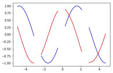
少し歯抜けの状態で、デモデータを作成して予測していきます。
demo_idices = [0, 13, 26, 39]  # デモデータのインデックス
for i in demo_idices:
    x_test = x_encoder[i:i+1] # 入力を一部取り出す(x_encoderは40.10,1の3次元配列で、1次元目がdemo_indicesの配列を10個取り出している)
    y_test = predict(x_test)

    plt.plot(axis_x[i:i+N_RNN], x_test.reshape(-1), color="b") # 変換前(青)
    plt.plot(axis_x[i:i+N_RNN], y_test, color="r") # 変換後(赤)

plt.show()
グラフにするとだいたい正弦関数が余弦関数に変換されているのがわかるかと思います。