目次
1.目的
2.対象
3.問題設定
4.検討に必要なライブラリ及び関数の定義
5.信号の定義
6.周波数変換1
7.dataの一部を削除(不等ピッチデータへの対応)
8.周波数変換2
9.まとめ
10.おまけ:周波数変換をする関数の紹介
11.追加検証
[1. 目的]
複数のセンサで取得した物理値をロガーで計測した際に、ロガーのサンプリングレートは固定にしているにもかかわらず、各センサの値に紐づくタイムスタンプは等間隔になっていないケースがあります。
通常、各センサ値を一つの共通したサンプリング間隔上で分析し、どの時間で何が起こっているかを各物理値を見て評価するため、タイムスタンプがずれているのは都合が悪いです。また、周波数解析も実施しづらくなってしまいます。
本記事では、上記のような状況に対応するために、周波数変換によるリサンプリング機能を実装し、タイムスタンプを再定義することに挑戦致します。
また、最後にはリサンプリングを1行で実行する関数を紹介しております。
私自身、まだまだ勉強中の身ですので、間違いなどありましたらご指摘頂けますと幸いです。
[2. 対象]
- 信号処理を活用するエンジニアや学生(音声、振動、生体、制御などの領域に関わる方々)
- 信号処理に興味のある方
[3. 問題設定]
本記事での一連の検討は「タイムスタンプを再定義しなければならない状況」を想定しています。
例えば、下記のような状況です。
- 不等ピッチに対するケアが必要
- ダウンサンプリング(間引き)して、データを軽くしたい
- アップサンプリング(補間)して、より細かい時間スケールの評価、周波数解析のためのデータ点数稼ぎなど
また、本検討はJupyter lab上で行いました。
[4. 検討に必要なライブラリ及び関数の定義]
まずは、必要なライブラリをインポートします。
今回、特に重要となるライブラリはscipyのinterpolateというモジュールです。
interpolateは周波数変換をする際の補間関数を定義してくれます。
# import setting
import numpy as np
import pandas as pd
import matplotlib.pyplot as plt
from scipy import interpolate
from scipy import signal
4-1. ローパスフィルタの実装
次にローパスフィルタを実行する関数を実装します。
データのアップサンプリング及びダウンサンプリングをする場合は、エイリアシングが発生するため適切なカットオフ周波数以下でローパスフィルタを適用する必要があります。
そこで、事前に下記のローパスフィルタを定義します。
ローパスフィルタの必要性に関しては、下記のURLが参考になるかもしれません。
[■参考: データ前処理のポイント ~ 振動データのダウンサンプリング https://www.macnica.co.jp/business/ai_iot/columns/133311/]
[■参考: サンプリング周波数変換 https://tetsufuku-blog.com/fs-convert/]
from scipy import signal
import matplotlib.pyplot as plt
import numpy as np

def butterlowpass(x, fpass, fstop, gpass, gstop, fs, dt, checkflag, labelname='Signal[-]'):
    '''
    バターワースを用いたローパスフィルタ
    filtfilt関数により位相ずれを防ぐ
    (順方向と逆方向からフィルタをかけて位相遅れを相殺)
    :param x: 入力データ
    :param fpass: 通過域端周波数[Hz]
    :param fstop: 阻止域端周波数[Hz]
    :param gpass: 通過域最大損失量[dB]
    :param gstop: 阻止域最大損失量[dB]
    :param fs: サンプリング周波数[Hz]
    :param dt: サンプリング間隔[s]
    :param checkflag: グラフ生成ON/OFF
    :param labelname: 信号ラベル名
    :return: フィルター後データ
    '''

    print('Applying filter against: {0}...'.format(labelname))
    fn = 1 / (2 * dt)
    Wp = fpass / fn
    Ws = fstop / fn
    N, Wn = signal.buttord(Wp, Ws, gpass, gstop)
    b1, a1 = signal.butter(N, Wn, "low")
    y = signal.filtfilt(b1, a1, x)
    print(y)

    if checkflag == True:
        time = np.arange(x.__len__()) * dt
        plt.figure(figsize = (12, 5))
        plt.title('Comparison between signals')
        plt.plot(time, x, color='black', label='Raw signal')
        plt.plot(time, y, color='red', label='Filtered signal')
        plt.xlabel('Time[s]')
        plt.ylabel(labelname)
        plt.show()
    return y
本関数は入力データ、通過域端周波数、阻止域端周波数、通過域最大損失量、阻止域最大損失量、サンプリング周波数とサンプリング間隔を用いてバターワースローパスフィルタを設計します。
この時、グラフ生成ONOFFフラグと信号ラベル名を補助情報として送ることでグラフを作成することが可能です。
しかし、本検討では使用いたしません。
また、この関数のポイントとしてfiltfilt関数を使用することでフィルタ適用による位相ずれをキャンセルいたします。
4-2. STFTの実装
次はSTFTを実装します。STFTは元の波形の信号分析及びアップサンプリング、ダウンサンプリングした結果の解析に使用いたします。
今回は下記のURLの内容を活用し、一部改造したものを使用しています。
■参考: PythonでFFT実装!SciPyのフーリエ変換まとめ https://watlab-blog.com/2019/04/21/python-fft/
# STFTを行う関数
# オーバーラップによる波形分割、窓関数適用と窓関数補正acfの適用、正規化及び平均化を行う

import numpy as np
from scipy import signal
from scipy import fftpack

def overlapping(data, samplerate, Fs, overlap_rate):
    '''
    入力データに対してオーバーラップ処理を行う
    フレームサイズを定義してデータを切り出すと切り出しができない部分が発生するため、
    切り出しができない部分の時間も返すように設定

    :param data: 入力データ
    :param samplerate: サンプリングレート[Hz]
    :param Fs: フレームサイズ
    :param overlap_rate: オーバーラップレート[%]

    :return:
        :array: オーバーラップ加工されたデータ
        :N_ave: オーバーラップ加工されたデータの個数
        :final_time: 最後に切り出したデータの時間
    '''
    Ts = len(data) / samplerate #入力データのデータ総点数
    Fc = Fs / samplerate #フレーム周期
    x_ol = Fs * (1 - (overlap_rate/100))#オーバーラップ時のフレームずらし幅
    N_ave = int((Ts - (Fc * (overlap_rate/100))) / (Fc * (1-(overlap_rate/100)))) #抽出するフレーム数(平均化に使うデータ個数)

    array = []#抽出したデータを格納する配列

    #forループでデータを抽出
    for i in range(N_ave):
        ps = int(x_ol * i) #切り出し開始位置を定義
        array.append(data[ps:ps+Fs:1])  #切り出し位置psからフレームサイズ分だけ抽出して配列に追加
    final_time = (ps + Fs) / samplerate
    return array, N_ave, final_time #オーバーラップ抽出されたデータ配列とデータ個数、最後に切り出したデータの時間を戻り値にする

# 窓関数処理
def window_func(data_array, Fs, N_ave, window_type):
    '''
    入力データに対して窓関数を適用する
    データ分割及びオーバーラップ処理で使用する。
    データを分割すると切り出した部分で波形が急に変化する。
    これを抑えるために窓関数を適用。
    ただし、窓関数を適用すると信号が減衰するため、補正処理を適用する
    :param data_array: 入力データ
    :param Fs: フレームサイズ
    :param N_ave: 分割データ数
    :param mode: 適用する窓関数の種類

    :return:
        :data_array: 窓関数が適用されたデータ
        :acf: 窓関数補正値
    '''
    if window_type == "hanning":
        window = signal.windows.hann(Fs)  # ハニング
    elif window_type == "hamming":
        window = signal.windows.hamming(Fs)# ハミング
    elif window_type == "blackman":
        window = signal.windows.blackman(Fs)  # ブラックマン
    elif window_type == "bartlett":
        window = signal.windows.bartlett(Fs)  # バートレット
    elif window_type == "kaiser":
        alpha = 0  # 0:矩形、1.5:ハミング、2.0:ハニング、3:ブラックマンに似た形
        Beta = np.pi * alpha
        window = signal.windows.kaiser(Fs, Beta)
    else:
        print("Error: input window function name is not supported. Your input was: ", window_type)
        print("Hanning window function is used.")
        window = signal.windows.hann(Fs)  # ハニング

    acf = 1 / (sum(window) / Fs)   #振幅補正係数(Amplitude Correction Factor)

    #オーバーラップされた複数時間波形全てに窓関数をかける
    for i in range(N_ave):
        data_array[i] = data_array[i] * window #窓関数をかける

    return data_array, acf


# FFT処理(平均化、正規化)
def fft_average(data_array,samplerate, Fs, N_ave, acf, spectrum_type):
    '''
    入力データのFFTを行い窓関数補正と正規化、平均化をする
    :param data_array:  入力データ
    :param samplerate: サンプリングレート、サンプリング周波数[Hz]
    :param Fs: フレームサイズ(FFTされるデータの点数)
    :param N_ave: フレーム総数
    :param acf:窓関数補正値
    :param mode: 解析モード


    :return:
        :fft_array: フーリエスペクトル(平均化、正規化及び窓補正済み)
        :fft_spectrum_mean_out: ナイキスト周波数まで抽出したスペクトル(スペクトルの種類は解析モードによる)
        :fft_axis_out: ナイキスト周波数まで抽出した周波数軸

    '''
    fft_array = []# フーリエスペクトルを格納する配列
    for i in range(N_ave):
        fft_array.append(acf*np.abs(fftpack.fft(data_array[i])/(Fs/2))) #FFTをして配列に追加、窓関数補正値をかけ、(Fs/2)の正規化を実施。さらに絶対値をとる

    fft_axis = np.linspace(0, samplerate, Fs)#周波数軸を作成
    fft_array = np.array(fft_array)#型をndarrayに変換

    if spectrum_type == "AMP":# 振幅スペクトルを求める場合
        amp_spectrum_mean = np.mean(fft_array, axis=0)# 平均化された振幅スペクトル

        #ナイキスト定数まで抽出
        fft_axis_out = fft_axis[:int(Fs / 2) + 1]
        fft_spectrum_mean_out = amp_spectrum_mean[:int(Fs // 2) + 1]

    elif spectrum_type == "PSD":# パワースペクトル密度を求める場合
        psd_spectrum_mean = np.mean(fft_array ** 2 / (samplerate / Fs), axis=0)  #平均化されたパワースペクトル密度
        # ナイキスト定数まで抽出
        fft_axis_out = fft_axis[:int(Fs / 2) + 1]
        fft_spectrum_mean_out = psd_spectrum_mean[:int(Fs // 2) + 1]

    else:
        print("Error: input fft mode name is not supported. Your input: ", spectrum_type)
        return -1

    return fft_array, fft_axis_out, fft_spectrum_mean_out


def STFT_main(t, data, Fs, samplerate, overlap_rate, window_type, spectrum_type):
    '''
    STFTを実施するメインコード
    :param t: 時間データ
    :param data: 時間データに対する信号のテータ
    :param Fs: フレームサイズ フレームサイズ = samplerate/周波数分解能
    :param samplerate: サンプリングレート[Hz]
    :param overlap_rate: オーバーラップ率[%]
    :param window_mode: 窓関数の種類
    :param analysis_mode: 解析モードの種類
    :return:
        :fft_array: フーリエスペクトル(平均化、正規化及び窓補正済み)
        :fft_spectrum_mean_out: ナイキスト周波数まで抽出したスペクトル(スペクトルの種類は解析モードによる)
        :fft_axis_out: ナイキスト周波数まで抽出した周波数軸

    '''
    print("Execute FFT")

    #入力データに対してオーバーラップ処理をする
    split_data, N_ave, final_time = overlapping(data, samplerate, Fs, overlap_rate)

    #窓関数を適用
    time_array, acf = window_func(split_data, Fs, N_ave, window_type=window_type)

    #FFTを実行
    fft_array, fft_axis_out, fft_spectrum_mean_out = fft_average(time_array, samplerate, Fs, N_ave, acf, spectrum_type)

    return fft_array, fft_axis_out, fft_spectrum_mean_out, final_time
少々長くなりましたが、上記がSTFTを実行するプログラムになります。
STFT_main関数を呼び出すことでオーバーラップ処理、窓関数適用、補正、平均化FFT及び正規化を実行します。
また、解析手法として、振幅スペクトル導出とパワースペクトル密度導出を選択できます。
上記二つの使い分け方として、連続周期信号の場合は振幅スペクトルやパワースペクトル、連続非周期信号の場合はパワースペクトル密度を使います。
■参考: 小野測器-FFT基本 FAQ https://www.onosokki.co.jp/HP-WK/c_support/faq/fft_common/fft_spectrum_13.htm
[5. 信号の定義]
さて、必要な関数は揃いましたので、次は信号を定義したいと思います。
今回は二つの信号を用意し、特性を下記のように定めました。
data1の特性
- サンプリング周波数samplerate = 100Hz
- 信号の周波数成分f1 = 2Hz、振幅 = 2
- 信号の周波数成分f2 = 4Hz、振幅 = 5
- 信号形状: f1及びf2の合成Sin波
- データ点数: 5000個(0 ~ 4999)
data2の特性
- サンプリング周波数samplerate = 100Hz
- 信号の周波数成分f3 = 5Hz、振幅 = 2
- 信号の周波数成分f4 = 20Hz、振幅 = 5
- 信号形状: f3及びf4の合成Sin波
- データ点数: 5000個(0 ~ 4999)
# 信号の生成
samplerate = 100
f1 = 2
f2 = 4
t = np.arange(0, 50, 1 / samplerate)
data1 = 2 * np.sin(2 * np.pi * f1 * t) + 5 * np.sin(2 * np.pi * f2 * t)


f3 = 5
f4 = 20
data2 = 2 * np.sin(2 * np.pi * f3 * t) + 5 * np.sin(2 * np.pi * f4 * t)

# DataFrame化
df = {}
df['Time'] = t
df['data1'] = data1
df['data2'] = data2
df = pd.DataFrame(df)

print(df.head())
print(df.tail())
df.shape
   Time     data1     data2
0  0.00  0.000000  0.000000
1  0.01  1.494116  5.373317
2  0.02  2.906148  4.114497
3  0.03  4.158985 -1.320892
4  0.04  5.185147 -2.853170
       Time     data1     data2
4995  49.95 -5.930853 -2.000000
4996  49.96 -5.185147  2.853170
4997  49.97 -4.158985  1.320892
4998  49.98 -2.906148 -4.114497
4999  49.99 -1.494116 -5.373317


(5000, 3)
定義したデータを下記でグラフ化します。
# グラフ化

fig, ax = plt.subplots(figsize = (16, 6))
ax.set_xlabel('Time[s]')
ax.set_ylabel('signal[-]')
ax.set_title('Original Data')

for label in df:
    if label != 'Time':
        ax.plot(df['Time'], df[label], label = label)
ax.legend(loc = 'upper right')
ax.set_xlim(0, 5)
ax.grid()
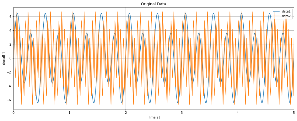
data2のほうがdata1よりも高周波成分を含むためノイジーになっています。
グラフ全体を表示すると分かりづらいため、今回は0 ~ 5sの間を表示しています。
[6.周波数変換1]
いよいよ、以降では周波数変換を実施します。
今回は、各dataをもとのサンプリング周波数からアップサンプリングし、次に元の周波数にダウンサンプリングします。
手順としては下記の通りです。
- 元のサンプリング周波数samplerateをf_temp = 1000Hzにアップサンプリング
- アップサンプリングされた信号に対して、samplerate / 2をカットオフ周波数として位相補償ローパスフィルタを適用
- ここでアップサンプリング処理が完了
- 次に、最終的に変換したいサンプリング周波数f_transにする前に、f_trans / 2をカットオフ周波数としてローパスフィルタを適用
- f_transにダウンサンプリングする
- ここでダウンサンプリング処理が完了
# 周波数変換のための設定
samplerate # もともとの信号のサンプリングレート(=100Hz)
f_temp = 1000# 1000Hzに変換することで汎用的にする
f_trans = 100# 最終的なサンプリング周波数
print('ベースサンプリング周波数' + str(samplerate) + 'Hz')
print('一時変換後のサンプリング周波数' + str(f_temp) + 'Hz')
print('最終的なサンプリング周波数' + str(f_trans) + 'Hz')
ベースサンプリング周波数100Hz
一時変換後のサンプリング周波数1000Hz
最終的なサンプリング周波数100Hz
6-1. アップサンプリング
周波数変換のための設定が完了したので、下記ではアップサンプリングをします。
元のサンプリング周波数は100Hzで、アップサンプリング後は1000Hzになります。
# アップサンプリング
# アップサンプリング後はアップサンプリング前のサンプリング周波数 / 2でLPFをかけてエイリアシングフィルタを適用
up_df = pd.DataFrame()
trans_nums = int((df['Time'].max() / (1 / samplerate)) * (f_temp / samplerate)) + 1# アップサンプリング後に必要なデータ点数を計算
print('アップサンプリング後のデータ点数: '+ str(trans_nums))
up_df['Time'] = np.linspace(0, max(df['Time']), trans_nums)# truns_nums個分のデータ点数を使用して等差級数を作成

# 各データラベル(ここではdata1とdata2)に対して補間関数を作成し、データをリサンプリング
for label in df:
    if label != 'Time':
        function = interpolate.interp1d(df['Time'], df[label], fill_value='extrapolate', kind = 'cubic')# 補間関数の作成
        up_df[label] = function(up_df['Time'])# リサンプリング
print(up_df.head())
print(up_df.tail())
print(up_df.shape)
アップサンプリング後のデータ点数: 49991
    Time     data1     data2
0  0.000  0.000000  0.000000
1  0.001  0.150855  0.856042
2  0.002  0.301600  1.639363
3  0.003  0.452156  2.350675
4  0.004  0.602443  2.990689
         Time     data1     data2
49986  49.986 -2.073538 -5.944820
49987  49.987 -1.930263 -5.967705
49988  49.988 -1.785887 -5.886060
49989  49.989 -1.640482 -5.690920
49990  49.990 -1.494116 -5.373317
(49991, 3)
ここでのポイントは二つあります。
一つ目は、補間関数に渡すデータ点数「trans_nums」の設定です。これは、周波数変換後の理想的なデータ点数を示しています。
例えば、今回の場合はサンプリング周波数100Hzで計測された0 ~ 49.99sのデータを1000Hzにアップサンプリングするため、5000個から49991個のデータ点数になります。
次に、interporate.inter1d関数についてです。この関数はサンプリングする部分を0埋めしたり、補間関数を線形・二次・三次などを指定できます。
この補間関数の設定は、リサンプリングの結果に大きな影響を及ぼします
ある計測信号に対して物理的・数学的にモデル(式)を定義できるのであれば、その理論式の次数や特性に応じて設定することをお勧めします。
詳しくはこちらをご覧ください。
■参考: scipy.interpolate.interp1d https://docs.scipy.org/doc/scipy/reference/generated/scipy.interpolate.interp1d.html
6-2. アンチエイリアシングフィルタの適用
アップサンプリング後は折り返し雑音(エイリアシング)が混入します。
そこで元のサンプリング周波数を1/2した値(ナイキスト周波数)でローパスフィルタをかけます。
これにより、アンチエイリアシングを施します。
また、ここではローパスフィルタのための関数「butterlowpass」を呼び出します。
この関数は、入力信号と通過域端周波数、阻止域端周波数、通過域最大損失量、阻止域最大損失量、サンプリング周波数とサンプリング間隔を用いてバターワースローパスフィルタを設計し、その関数を入力信号に適用します。
下記のURLが非常に参考になります。
■参考URL:PythonのSciPyでローパスフィルタをかける! https://watlab-blog.com/2019/04/30/scipy-lowpass/#383062596812501124491245212523
# ローパスフィルタ適用<エイリアシングフィルタ>
# アップサンプリング後のLPFなのでカットオフ周波数はもとの信号のサンプリング周波数の1/2にすること

labellist = up_df.columns[1:].to_list()# 解析したい信号のラベルを抽出
filtered_up_df = pd.DataFrame()
filtered_up_df['Time'] = up_df['Time']
for idx, labelname in enumerate(labellist):
    filtered_up_df[labelname] = butterlowpass(x=up_df[labelname], fpass=int(samplerate / 2.56),
                                                            fstop=int(samplerate / 2),
                                                            gpass=3,
                                                            gstop=70,
                                                            fs=samplerate,
                                                            dt=1 / samplerate,
                                                            checkflag=False,
                                                            labelname=labelname)

print(filtered_up_df.head())
print(filtered_up_df.describe)
print(filtered_up_df.shape)
Applying filter against: data1...
[ 1.47162637e-04  1.50781612e-01  3.01626685e-01 ... -1.78592211e+00
 -1.64030675e+00 -1.49439254e+00]
Applying filter against: data2...
[ 4.46247898e-04  8.52369717e-01  1.63766668e+00 ... -5.88323419e+00
 -5.68520048e+00 -5.37283111e+00]
    Time     data1     data2
0  0.000  0.000147  0.000446
1  0.001  0.150782  0.852370
2  0.002  0.301627  1.637667
3  0.003  0.452131  2.348081
4  0.004  0.602439  2.988551
<bound method NDFrame.describe of          Time     data1     data2
0       0.000  0.000147  0.000446
1       0.001  0.150782  0.852370
2       0.002  0.301627  1.637667
3       0.003  0.452131  2.348081
4       0.004  0.602439  2.988551
...       ...       ...       ...
49986  49.986 -2.073516 -5.941923
49987  49.987 -1.930196 -5.963940
49988  49.988 -1.785922 -5.883234
49989  49.989 -1.640307 -5.685200
49990  49.990 -1.494393 -5.372831

[49991 rows x 3 columns]>
(49991, 3)
6-3. 時系列データの確認
ここで、元のデータ、アップサンプリング後のデータ、ローパスフィルタ適用後のデータを比較してみます。
# グラフ化

fig, ax = plt.subplots(figsize = (16, 6))
ax.set_xlabel('Time[s]')
ax.set_ylabel('signal[-]')
ax.set_title('Original data1 vs UpSampling data1 vs Filtered UpSampling data1')
ax.plot(df['Time'], df['data1'], label = 'Original data1', marker = 'D')
ax.plot(up_df['Time'], up_df['data1'], label = 'UpSampling data1', marker='*')
ax.plot(filtered_up_df['Time'], filtered_up_df['data1'], label = 'Filtered UpSampling data1', marker = '+')

ax.legend(loc = 'upper right')
ax.set_xlim(0, 10 * (1 / samplerate))
ax.grid()


fig, ay = plt.subplots(figsize = (16, 6))
ay.set_xlabel('Time[s]')
ay.set_ylabel('signal[-]')
ay.set_title('Original data2 vs UpSampling data2 vs Filtered UpSampling data2')
ay.plot(df['Time'], df['data2'], label = 'Original data2', marker = 'D')
ay.plot(up_df['Time'], up_df['data2'], label = 'UpSampling data2', marker='*')
ay.plot(filtered_up_df['Time'], filtered_up_df['data2'], label = 'Filtered Up Sampling data2', marker = '+')
ay.legend(loc = 'upper right')
ay.set_xlim(0, 10 * (1 / samplerate))
ay.grid()
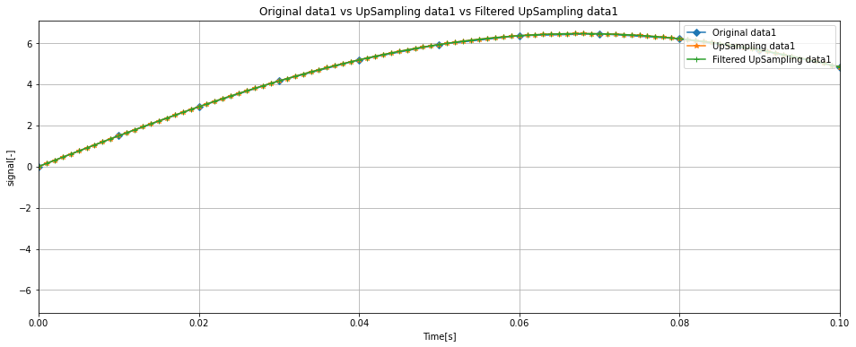
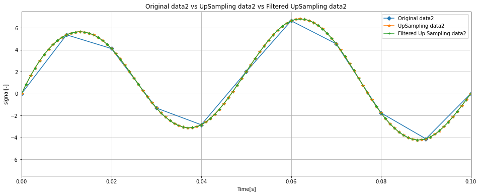
data1、data2ともに波形の傾向はつかめているようです。
また、アップサンプリング後とフィルタ適用後の波形に大きな違いはなさそうです。
6-4.周波数スペクトルの確認(オリジナルデータ / アップサンプリング後のデータ / アップサンプリング後にフィルタを適用したデータ)
下記では各データに対してSTFTを適用し、スペクトルの確認をします。
# STFTをしてスペクトル解析をする

# オリジナルデータ
delta_f = 0.2# 周波数分解能(自分で決める)
Fs = int(samplerate / delta_f)
print(delta_f, samplerate, Fs, Fs/samplerate)
overlap_rate = 70  # オーバーラップ率
fft_array_data1, fft_axis_data1, fft_spectrum_data1, final_time_data1 = STFT_main(df['Time'].to_list(), df['data1'].to_list(), Fs, samplerate, overlap_rate, window_type="hanning", spectrum_type="AMP")
fft_array_data2, fft_axis_data2, fft_spectrum_data2, final_time_data2 = STFT_main(df['Time'].to_list(), df['data2'].to_list(), Fs, samplerate, overlap_rate, window_type="hanning", spectrum_type="AMP")
0.2 100 500 5.0
Execute FFT
Execute FFT
# STFTをしてスペクトル解析をする
# アップサンプリングデータ

delta_f = 0.2# 周波数分解能(自分で決める)
Fs = int(f_temp / delta_f)
print(delta_f, f_temp, Fs, Fs/f_temp)
overlap_rate = 70  # オーバーラップ率
fft_array_up_data1, fft_axis_up_data1, fft_spectrum_up_data1, final_time_up_data1 = STFT_main(up_df['Time'].to_list(), up_df['data1'].to_list(), Fs, f_temp, overlap_rate, window_type="hanning", spectrum_type="AMP")
fft_array_up_data2, fft_axis_up_data2, fft_spectrum_up_data2, final_time_up_data2 = STFT_main(up_df['Time'].to_list(), up_df['data2'].to_list(), Fs, f_temp, overlap_rate, window_type="hanning", spectrum_type="AMP")
0.2 1000 5000 5.0
Execute FFT
Execute FFT
# アップサンプリングデータ(1000Hzにアップサンプリング)に対してローパスフィルタをかけたデータ

delta_f = 0.2# 周波数分解能(自分で決める)
Fs = int(f_temp / delta_f)
print(delta_f, f_temp, Fs, Fs/f_temp)
overlap_rate = 70  # オーバーラップ率
fft_array_filt_data1, fft_axis_filt_data1, fft_spectrum_filt_data1, final_time_filt_data1 = STFT_main(filtered_up_df['Time'].to_list(), filtered_up_df['data1'].to_list(), Fs, f_temp, overlap_rate, window_type="hanning", spectrum_type="AMP")
fft_array_filt_data2, fft_axis_filt_data2, fft_spectrum_filt_data2, final_filt_up_data2 = STFT_main(filtered_up_df['Time'].to_list(), filtered_up_df['data2'].to_list(), Fs, f_temp, overlap_rate, window_type="hanning", spectrum_type="AMP")
0.2 1000 5000 5.0
Execute FFT
Execute FFT
# 三つのデータの比較
fig, ax = plt.subplots(figsize = (16, 6))
ax.set_xlabel('f[Hz]')
ax.set_ylabel('Amplitude[v]')
ax.set_title('Comparison of data1')
ax.plot(fft_axis_data1, fft_spectrum_data1, label = 'Original data1', marker = 'D')
ax.plot(fft_axis_up_data1, fft_spectrum_up_data1, label = 'UpSampling data1', marker = '*')
ax.plot(fft_axis_filt_data1, fft_spectrum_filt_data1, label = 'Filtered UpSampling data1', marker = '+')
ax.legend(loc = 'upper right')
ax.set_xlim(0, 10)
ax.grid()


fig, ay = plt.subplots(figsize = (16, 6))
ay.set_xlabel('f[Hz]')
ay.set_ylabel('Amplitude[v]')
ay.set_title('Comparison of data2')
ay.plot(fft_axis_data2, fft_spectrum_data2, label = 'Original data2', marker = '*')
ay.plot(fft_axis_up_data2, fft_spectrum_up_data2, label = 'UpSampling data2', marker = '*')
ay.plot(fft_axis_filt_data2, fft_spectrum_filt_data2, label = 'Filtered UpSampling data2', marker = '+')

ay.legend(loc = 'upper right')
ay.set_xlim(0, 30)
ay.grid()
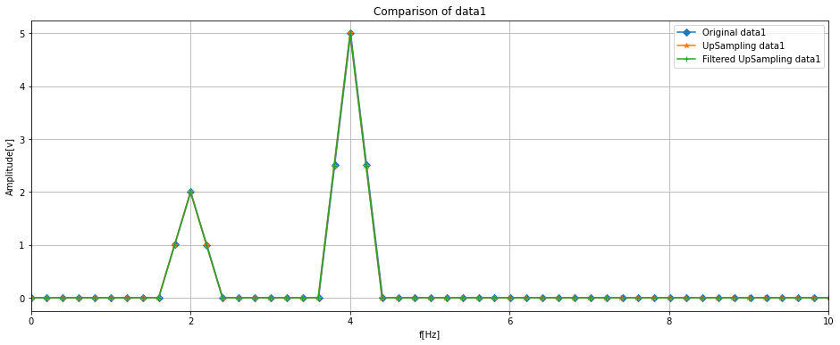
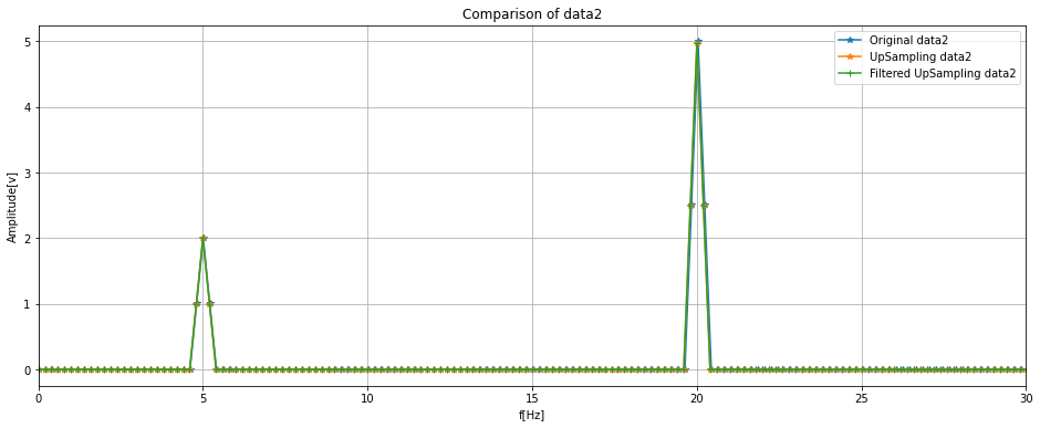
data1について、周波数成分は2Hzと4Hzで振幅がそれぞれ2と5です。
振幅スペクトルを確認するとデータ加工後も正しくスペクトルが得られているのが分かります
data2については、5Hzと20Hzの周波数成分を持ち、振幅はそれぞれ2と5です。
スペクトルの傾向としてはdata1と同様に良好そうです。
6-5. ダウンサンプリング前のアンチエイリアシングフィルタ適用
ここまでで、アップサンプリングとアンチエイリアシングフィルタの適用が完了しました。
次に、最終的に変換したい周波数にするためにダウンサンプリングをします。
ダウンサンプリングの際は、ダウンサンプリングする前に、変換後のサンプリング周波数の1/2でローパスフィルタをかけます。
# ダウンサンプリング前のアンチエイリアシング処理
# 変換したい周波数のナイキスト周波数をカットオフにしてLPF
labellist = filtered_up_df.columns[1:].to_list()# 解析したい信号のラベルを抽出
filtered_df = pd.DataFrame()
filtered_df['Time'] = filtered_up_df['Time']
for idx, labelname in enumerate(labellist):
    filtered_df[labelname] = butterlowpass(x=filtered_up_df[labelname], fpass=int(f_trans / 2.56),
                                                            fstop=int(f_trans / 2),
                                                            gpass=3,
                                                            gstop=30,
                                                            fs=f_temp,
                                                            dt=1 / f_temp,
                                                            checkflag=False,
                                                            labelname=labelname)

print(filtered_df.head())
print(filtered_df.describe)
print(filtered_df.shape)
Applying filter against: data1...
[ 0.00678001  0.15770432  0.30813447 ... -1.6151652  -1.46589898
 -1.3241629 ]
Applying filter against: data2...
[ 0.0682752   0.76911476  1.45579839 ... -5.79091745 -5.91894179
 -6.02545672]
    Time     data1     data2
0  0.000  0.006780  0.068275
1  0.001  0.157704  0.769115
2  0.002  0.308134  1.455798
3  0.003  0.458024  2.118544
4  0.004  0.607345  2.748068
<bound method NDFrame.describe of          Time     data1     data2
0       0.000  0.006780  0.068275
1       0.001  0.157704  0.769115
2       0.002  0.308134  1.455798
3       0.003  0.458024  2.118544
4       0.004  0.607345  2.748068
...       ...       ...       ...
49986  49.986 -1.931372 -5.459798
49987  49.987 -1.770769 -5.638725
49988  49.988 -1.615165 -5.790917
49989  49.989 -1.465899 -5.918942
49990  49.990 -1.324163 -6.025457

[49991 rows x 3 columns]>
(49991, 3)
6-6. ダウンサンプリング
ローパスフィルタ適用後にダウンサンプリングします。
# アップサンプリングしたデータをダウンサンプリングする処理
down_df = pd.DataFrame()
trans_nums = int((filtered_df['Time'].max() / (1 / f_temp)) * (f_trans / f_temp)) + 1
down_df['Time'] = np.linspace(0, max(filtered_df['Time']), trans_nums)

for label in filtered_up_df:
    if label != 'Time':
        function = interpolate.interp1d(filtered_df['Time'], filtered_df[label], fill_value = 'extrapolate', kind = 'cubic')
        down_df[label] = function(down_df['Time'])
print(down_df.head())
print(down_df.tail())
print(down_df.shape)
   Time     data1     data2
0  0.00  0.006780  0.068275
1  0.01  1.491107  5.399231
2  0.02  2.904238  4.074774
3  0.03  4.159400 -1.298575
4  0.04  5.180590 -2.827840
       Time     data1     data2
4995  49.95 -5.955261 -1.986663
4996  49.96 -5.136238  2.910250
4997  49.97 -4.200735  1.089634
4998  49.98 -2.918014 -3.721232
4999  49.99 -1.324163 -6.025457
(5000, 3)
6-7. 時系列グラフの確認(オリジナルデータ / アップサンプリング後のデータ / アップサンプリング後にフィルタを適用したデータ / ダウンサンプリング前にフィルタを適用したデータ / ダウンサンプリング後のデータ)
これですべての処理が完了しました。そこで、全てのデータに対して時系列グラフを観察してみます。
# グラフ化

fig, ax = plt.subplots(figsize = (16, 6))
ax.set_xlabel('Time[s]')
ax.set_ylabel('signal[-]')
ax.set_title('Comparison of data1')
ax.plot(df['Time'], df['data1'], label = 'Original data1', marker = 'D')
ax.plot(up_df['Time'], up_df['data1'], label = 'UpSampling data1', marker='*')
ax.plot(filtered_up_df['Time'], filtered_up_df['data1'], label = 'Filtered UpSampling data1', marker = '+')
ax.plot(filtered_df['Time'], filtered_df['data1'], label = 'Filtered before DownSampling data1', marker = 'v')
ax.plot(down_df['Time'], down_df['data1'], label = 'DownSampling data1', marker = '<')


ax.legend(loc = 'upper right')
ax.set_xlim(0, 10 * (1 / f_trans))
ax.grid()


fig, ay = plt.subplots(figsize = (16, 6))
ay.set_xlabel('Time[s]')
ay.set_ylabel('signal[-]')
ay.set_title('Comparison of data2')
ay.plot(df['Time'], df['data2'], label = 'Original data2', marker = 'D')
ay.plot(up_df['Time'], up_df['data2'], label = 'UpSampling data2', marker='*')
ay.plot(filtered_up_df['Time'], filtered_up_df['data2'], label = 'Filtered UpSampling data2', marker = '+')
ay.plot(filtered_df['Time'], filtered_df['data2'], label = 'Filtered before DownSampling data2', marker = 'v')
ay.plot(down_df['Time'], down_df['data2'], label = 'DownSampling data2', marker = '<')
ay.legend(loc = 'upper right')
ay.set_xlim(0, 10 * (1 / f_trans))
ay.grid()

fig, az = plt.subplots(figsize = (16, 6))
az.set_xlabel('Time[s]')
az.set_ylabel('signal[-]')
az.set_title('Original data vs final result(DownSampling data)')
az.plot(df['Time'], df['data1'], label = 'Original data1', marker = 'D')
az.plot(down_df['Time'], down_df['data1'], label = 'final result data1', marker='*')
az.plot(df['Time'], df['data2'], label = 'Original data2', marker = 'v')
az.plot(down_df['Time'], down_df['data2'], label = 'final result data1', marker='<')
az.set_xlim(0, 10 * (1 / f_trans))
az.grid()
az.legend(loc = 'upper right')
az.set_xlim(0, 10 * (1 / f_trans))
(0.0, 0.1)
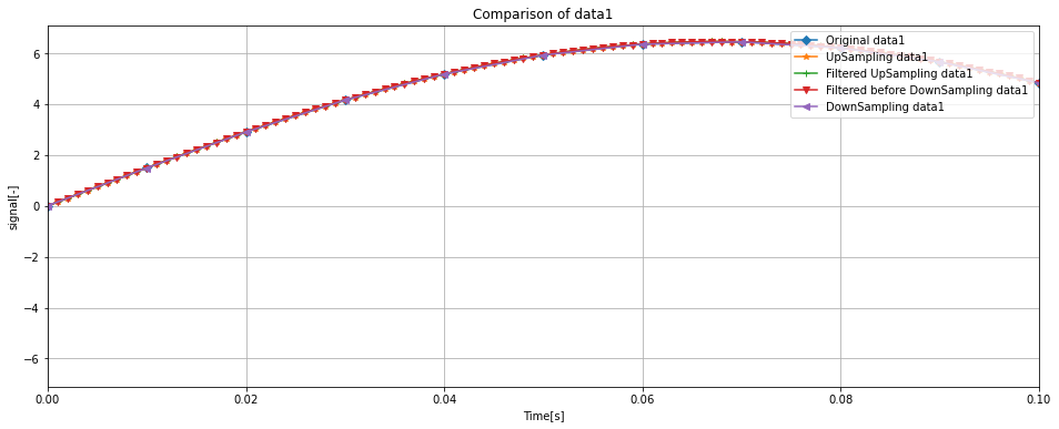
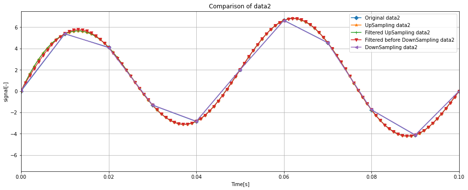
一つ目のグラフはdata1について全ての処理結果を示したグラフ、二つ目のグラフはdata2について全ての処理結果を示したグラフになります。
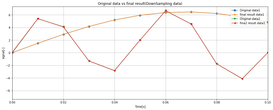
また、三つ目のグラフはオリジナルのデータと最終的なデータのみにフォーカスしたデータです。
オリジナルのデータに対して最終的なデータがしっかりと傾向をつかめているのが分かります。
6-8. 周波数スペクトルの確認(オリジナルデータ / アップサンプリング後のデータ / アップサンプリング後にフィルタを適用したデータ / ダウンサンプリング前にフィルタを適用したデータ / ダウンサンプリング後のデータ)
最後に全ての加工データのスペクトル解析します。
# ダウンサンプリング前にフィルタを適用したデータの周波数解析
delta_f = 0.2# 周波数分解能(自分で決める)
Fs = int(f_temp / delta_f)
overlap_rate = 70  # オーバーラップ率
fft_array_filtered_data1, fft_axis_filtered_data1, fft_spectrum_filtered_data1, final_time_filtered_data1 = STFT_main(filtered_df['Time'].to_list(), filtered_df['data1'].to_list(), Fs, f_temp, overlap_rate, window_type="hanning", spectrum_type="AMP")
fft_array_filtered_data2, fft_axis_filtered_data2, fft_spectrum_filtered_data2, final_time_filtered_data2 = STFT_main(filtered_df['Time'].to_list(), filtered_df['data2'].to_list(), Fs, f_temp, overlap_rate, window_type="hanning", spectrum_type="AMP")
Execute FFT
Execute FFT
# ダウンサンプリング後データの周波数解析
delta_f = 0.2# 周波数分解能(自分で決める)
Fs = int(f_trans / delta_f)
overlap_rate = 70  # オーバーラップ率
fft_array_down_data1, fft_axis_down_data1, fft_spectrum_down_data1, final_time_down_data1 = STFT_main(down_df['Time'].to_list(), down_df['data1'].to_list(), Fs, f_trans, overlap_rate, window_type="hanning", spectrum_type="AMP")
fft_array_down_data2, fft_axis_down_data2, fft_spectrum_down_data2, final_time_down_data2 = STFT_main(down_df['Time'].to_list(), down_df['data2'].to_list(), Fs, f_trans, overlap_rate, window_type="hanning", spectrum_type="AMP")
Execute FFT
Execute FFT
# 全データの周波数解析結果の比較
fig, ax = plt.subplots(figsize = (16, 6))
ax.set_xlabel('f[Hz]')
ax.set_ylabel('Amplitude[v]')
ax.set_title('Comparison of data1')
ax.plot(fft_axis_data1, fft_spectrum_data1, label = 'Original data1', marker = 'D')
ax.plot(fft_axis_up_data1, fft_spectrum_up_data1, label = 'UpSampling data1', marker = '*')
ax.plot(fft_axis_filt_data1, fft_spectrum_filt_data1, label = 'Filtered UpSampling data1', marker = '+')
ax.plot(fft_axis_filtered_data1, fft_spectrum_filtered_data1, label = 'Filter before DownSampling data1', marker = 'v')
ax.plot(fft_axis_filtered_data1, fft_spectrum_filtered_data1, label = 'DownSampling data1', marker = '<')


ax.legend(loc = 'upper right')
ax.set_xlim(0, 10)
ax.grid()


fig, ay = plt.subplots(figsize = (16, 6))
ay.set_xlabel('f[Hz]')
ay.set_ylabel('Amplitude[v]')
ay.set_title('Comparison of data2')
ay.plot(fft_axis_data2, fft_spectrum_data2, label = 'Original data2', marker = 'D')
ay.plot(fft_axis_up_data2, fft_spectrum_up_data2, label = 'UpSampling data2', marker = '*')
ay.plot(fft_axis_filt_data2, fft_spectrum_filt_data2, label = 'Filtered UpSampling data2', marker = '+')
ay.plot(fft_axis_filtered_data2, fft_spectrum_filtered_data2, label = 'Filter before DownSampling data2', marker = 'v')
ay.plot(fft_axis_down_data2, fft_spectrum_down_data2, label = 'DownSampling data2', marker = '<')

ay.legend(loc = 'upper right')
ay.set_xlim(0, 30)
ay.grid()
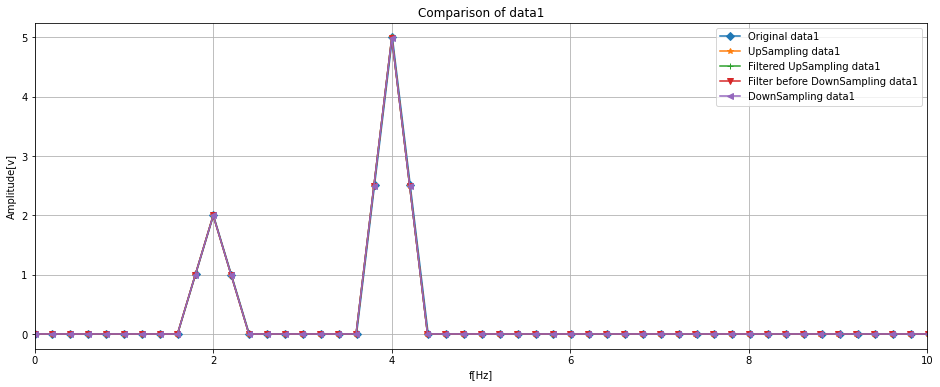
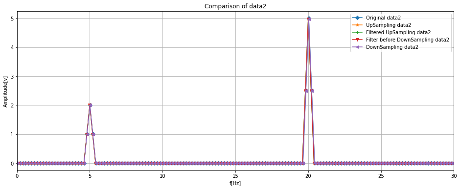
周波数分析した結果でも、オリジナルのデータに対して最終的なデータが特徴をつかんでいるのが分かります。
まとめると、下記のようになります。
- ある信号において、周波数Aから周波数Bへの変換はintepolate関数を活用するとよい。
- ただし、補間の設定は理論式に基づき実施する必要がある。
- リサンプリングをする際は、適切なタイミング及び適切な周波数でローパスフィルタをかけてアンチエイリアシングをする。
[7. dataの一部を削除(不等ピッチデータへの対応)]
さて、本当に対応したいのは不等ピッチのデータです。
そこで、data1、data2を下記のように変更しました。
- ランダムなポイントでロガーでの計測がされないケースを想定し、ランダムに行を削除
そこで、500個のデータをもとのデータフレームdfからdropしました。
これにより、一様なサンプリングで取得されていないデータが疑似的に作ることが出来ました。
すなわち、データロガーでは0.01sでサンプリングしているにも関わらず、0.02や0.05sごとにタイムスタンプが切れている現象が起きえます。
np.random.seed(seed=100)
rand = (4999 - 1) * np.random.rand(500) + 1
print('Drop ' + str(len(rand)) +' samples')
rand = [int(val) for val in rand]
dirty_df = df.drop(df.index[rand])
Drop 500 samples
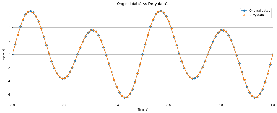
グラフ化すると下記のようになります。
fig, ax = plt.subplots(figsize = (16, 6))
ax.set_xlabel('Time[s]')
ax.set_ylabel('signal[-]')
ax.set_title('Original data1 vs Dirty data1')
ax.plot(df['Time'], df['data1'], label = 'Original data1', marker = 'D')
ax.plot(dirty_df['Time'], dirty_df['data1'], label = 'Dirty data1', marker='*')
ax.legend(loc = 'upper right')
ax.set_xlim(0, 100 * (1 / samplerate))
ax.grid()

fig, ax = plt.subplots(figsize = (16, 6))
ax.set_xlabel('Time[s]')
ax.set_ylabel('signal[-]')
ax.set_title('Original data2 vs Dirty data2')
ax.plot(df['Time'], df['data2'], label = 'Original data2', marker = 'D')
ax.plot(dirty_df['Time'], dirty_df['data2'], label = 'Dirty data2', marker='*')
ax.legend(loc = 'upper right')
ax.set_xlim(0, 100 * (1 / samplerate))
ax.grid()

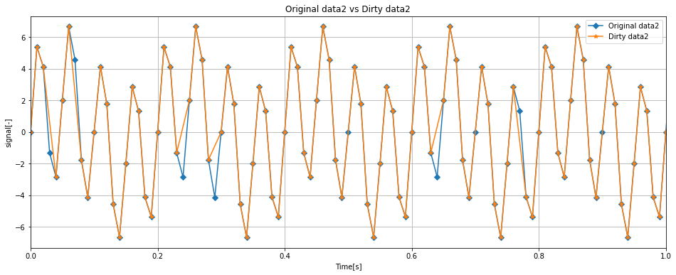
オリジナルデータに対してDirty dataはいくつかのプロットが喪失したデータとなりました。
この時の周波数解析結果を見てみたいと思います。
#  一様にサンプリングされていないdata(dirty)のSTFT
delta_f = 0.2# 周波数分解能(自分で決める)
Fs = int(samplerate / delta_f)
overlap_rate = 70  # オーバーラップ率
fft_array_dirty_data1, fft_axis_dirty_data1, fft_spectrum_dirty_data1, final_time_dirty_data1 = STFT_main(dirty_df['Time'].to_list(), dirty_df['data1'].to_list(), Fs, samplerate, overlap_rate, window_type="hanning", spectrum_type="AMP")
fft_array_dirty_data2, fft_axis_dirty_data2, fft_spectrum_dirty_data2, final_time_dirty_data2 = STFT_main(dirty_df['Time'].to_list(), dirty_df['data2'].to_list(), Fs, samplerate, overlap_rate, window_type="hanning", spectrum_type="AMP")
Execute FFT
Execute FFT
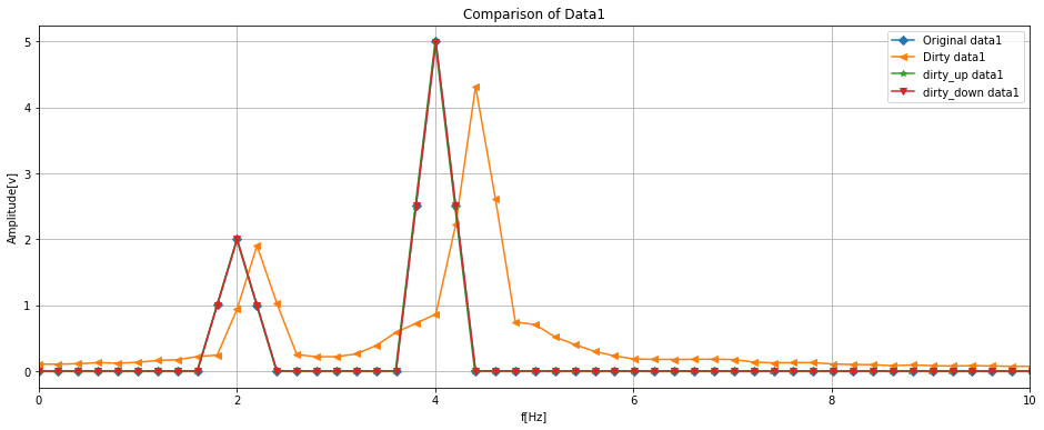
fig, ax = plt.subplots(figsize = (16, 6))
ax.set_xlabel('f[Hz]')
ax.set_ylabel('Amplitude[v]')
ax.set_title('Comparison of Data1')
ax.plot(fft_axis_data1, fft_spectrum_data1, label = 'Original data1', marker = 'D')
ax.plot(fft_axis_dirty_data1, fft_spectrum_dirty_data1, label = 'Dirty data1', marker = '<')


ax.legend(loc = 'upper right')
ax.set_xlim(0, 10)
ax.grid()


fig, ay = plt.subplots(figsize = (16, 6))
ay.set_xlabel('f[Hz]')
ay.set_ylabel('Amplitude[v]')
ay.set_title('Comparison of Data2')
ay.plot(fft_axis_data2, fft_spectrum_data2, label = 'Original data2', marker = 'D')
ay.plot(fft_axis_dirty_data2, fft_spectrum_dirty_data2, label = 'Dirty data2', marker = '<')

ay.legend(loc = 'upper right')
ay.set_xlim(0, 30)
ay.grid()
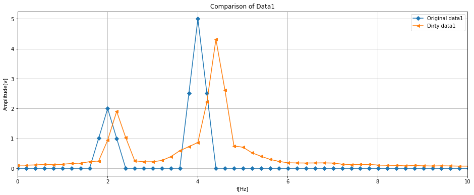
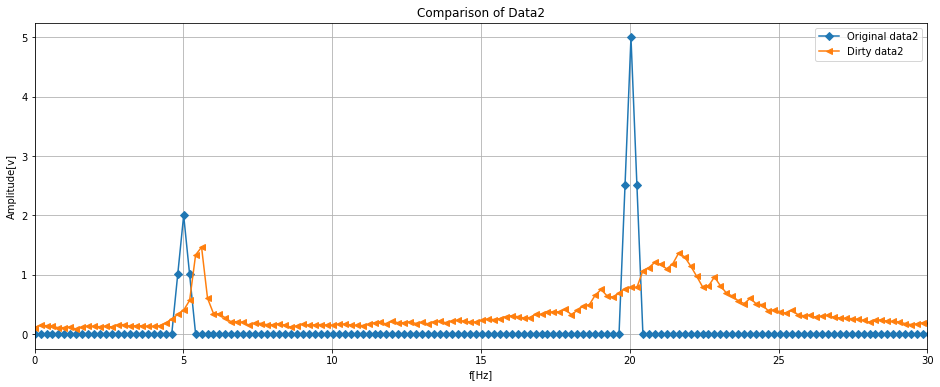
さて、周波数解析をした結果、真の信号であるオリジナルに対して、オリジナルから一部の情報を消したDirty(すなわち一様にサンプリングされていないデータ)は信号の特性がかなり変わったものとなりました。
Data1はピーク周波数がずれ、Data2はピーク周波数の裾野がかなり広がっています。
こちらを6章までに取り上げた内容でオリジナルデータに復元できるかを試してみます。
[8. 周波数変換2]
一度現状を整理します。
- サンプリング周波数100Hzでデータを計測した
- タイムスタンプが0.01sずつ記録されるはずだが、何らかの原因で0.01sの次が0.03sといったように不等ピッチになっている
これらのデータに対して、一度1000Hzにアップサンプリングしてから100Hzにダウンサンプリングします。
# アップサンプリング
# アップサンプリング後はアップサンプリング前のサンプリング周波数 / 2でLPFをかけてエイリアシングフィルタを適用
up_dirty_df = pd.DataFrame()
trans_nums = int((dirty_df['Time'].max() / (1 / samplerate)) * (f_temp / samplerate)) + 1# アップサンプリング後に必要なデータ点数を計算
print('アップサンプリング後のデータ点数: '+ str(trans_nums))
up_dirty_df['Time'] = np.linspace(0, max(dirty_df['Time']), trans_nums)# truns_nums個分のデータ点数を使用して等差級数を作成
up_dirty_df.head()

# 各データラベル(ここではdata1とdata2)に対して補間関数を作成し、データをリサンプリング
for label in dirty_df:
    if label != 'Time':
        function = interpolate.interp1d(dirty_df['Time'], dirty_df[label], fill_value = 'extrapolate', kind = 'cubic')# 補間関数の作成
        up_dirty_df[label] = function(up_dirty_df['Time'])# リサンプリング
アップサンプリング後のデータ点数: 49991
# アップサンプリング後の時系列のサンプリング間隔確認
print(up_dirty_df.head())
print(up_dirty_df.tail())
print(up_dirty_df.shape)
    Time     data1     data2
0  0.000  0.000000  0.000000
1  0.001  0.150786  0.899369
2  0.002  0.301484  1.712335
3  0.003  0.452011  2.441130
4  0.004  0.602288  3.087984
         Time     data1     data2
49986  49.986 -2.073543 -5.946442
49987  49.987 -1.930267 -5.969213
49988  49.988 -1.785891 -5.887277
49989  49.989 -1.640484 -5.691642
49990  49.990 -1.494116 -5.373317
(49991, 3)
# ローパスフィルタ適用<エイリアシングフィルタ>
# アップサンプリング後のLPFなのでカットオフ周波数はもとの信号のサンプリング周波数の1/2にすること

labellist = df.columns[1:].to_list()# 解析したい信号のラベルを抽出
filtered_up_dirty_df = pd.DataFrame()
filtered_up_dirty_df['Time'] = up_dirty_df['Time']
for idx, labelname in enumerate(labellist):
    filtered_up_dirty_df[labelname] = butterlowpass(x=up_dirty_df[labelname], fpass=int(samplerate / 2.56),
                                                            fstop=int(samplerate / 2),
                                                            gpass=3,
                                                            gstop=70,
                                                            fs=samplerate,
                                                            dt=1 / samplerate,
                                                            checkflag=False,
                                                            labelname=labelname)
Applying filter against: data1...
[ 1.47185165e-04  1.50713694e-01  3.01510967e-01 ... -1.78592542e+00
 -1.64030870e+00 -1.49439254e+00]
Applying filter against: data2...
[ 4.32097505e-04  8.95031025e-01  1.71035218e+00 ... -5.88444627e+00
 -5.68591201e+00 -5.37283067e+00]
fig, ax = plt.subplots(figsize = (16, 6))
ax.set_xlabel('Time[s]')
ax.set_ylabel('signal[-]')
ax.set_title('Original data1 vs Dirty data1')
ax.plot(df['Time'], df['data1'], label = 'Original data1', marker = 'D')
ax.plot(dirty_df['Time'], dirty_df['data1'], label = 'Dirty data1', marker='*')
ax.plot(filtered_up_dirty_df['Time'], filtered_up_dirty_df['data1'], label = 'Dirty filterd upsampling1', marker='+')
ax.legend(loc = 'upper right')
ax.set_xlim(0, 100 * (1 / samplerate))
ax.grid()

fig, ax = plt.subplots(figsize = (16, 6))
ax.set_xlabel('Time[s]')
ax.set_ylabel('signal[-]')
ax.set_title('Original data2 vs Dirty data2')
ax.plot(df['Time'], df['data2'], label = 'Original data2', marker = 'D')
ax.plot(dirty_df['Time'], dirty_df['data2'], label = 'Dirty data2', marker='*')
ax.plot(filtered_up_dirty_df['Time'], filtered_up_dirty_df['data2'], label = 'Dirty filterd upsampling2', marker='+')
ax.legend(loc = 'upper right')
ax.set_xlim(0, 100 * (1 / samplerate))
ax.grid()
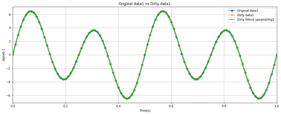
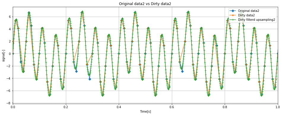
Dirty dataに対して1000Hzのアップサンプリングを適用した結果、Originalにだいぶ近づきました。
これなら波形の傾向はつかめそうです。
# ダウンサンプリング前のアンチエイリアシング処理
# 変換したい周波数のナイキスト周波数をカットオフにしてLPF
labellist = filtered_up_dirty_df.columns[1:].to_list()# 解析したい信号のラベルを抽出
filtered_dirty_df = pd.DataFrame()
filtered_dirty_df['Time'] = filtered_up_dirty_df['Time']
for idx, labelname in enumerate(labellist):
    filtered_dirty_df[labelname] = butterlowpass(x=filtered_up_dirty_df[labelname], fpass=int(f_trans / 2.56),
                                                            fstop=int(f_trans / 2),
                                                            gpass=3,
                                                            gstop=30,
                                                            fs=f_temp,
                                                            dt=1 / f_temp,
                                                            checkflag=False,
                                                            labelname=labelname)

print(filtered_dirty_df.head())
print(filtered_dirty_df.describe)
filtered_df['Time']
Applying filter against: data1...
[ 0.00659322  0.1575289   0.30797218 ... -1.61483223 -1.46557274
 -1.32384659]
Applying filter against: data2...
[ 0.08117396  0.77522691  1.45423057 ... -5.779604   -5.90508845
 -6.00958512]
    Time     data1     data2
0  0.000  0.006593  0.081174
1  0.001  0.157529  0.775227
2  0.002  0.307972  1.454231
3  0.003  0.457875  2.108409
4  0.004  0.607210  2.728592
<bound method NDFrame.describe of          Time     data1     data2
0       0.000  0.006593  0.081174
1       0.001  0.157529  0.775227
2       0.002  0.307972  1.454231
3       0.003  0.457875  2.108409
4       0.004  0.607210  2.728592
...       ...       ...       ...
49986  49.986 -1.931036 -5.455030
49987  49.987 -1.770433 -5.630456
49988  49.988 -1.614832 -5.779604
49989  49.989 -1.465573 -5.905088
49990  49.990 -1.323847 -6.009585

[49991 rows x 3 columns]>


0         0.000
1         0.001
2         0.002
3         0.003
4         0.004
          ...
49986    49.986
49987    49.987
49988    49.988
49989    49.989
49990    49.990
Name: Time, Length: 49991, dtype: float64
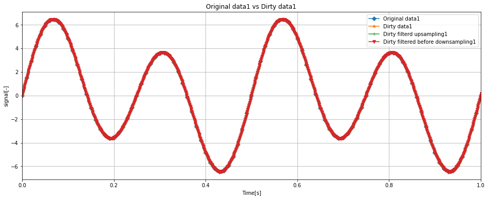
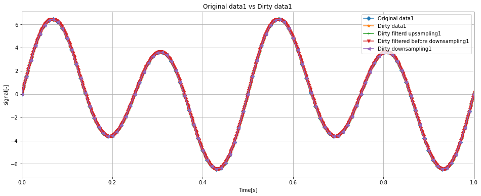
fig, ax = plt.subplots(figsize = (16, 6))
ax.set_xlabel('Time[s]')
ax.set_ylabel('signal[-]')
ax.set_title('Original data1 vs Dirty data1')
ax.plot(df['Time'], df['data1'], label = 'Original data1', marker = 'D')
ax.plot(dirty_df['Time'], dirty_df['data1'], label = 'Dirty data1', marker='*')
ax.plot(filtered_up_dirty_df['Time'], filtered_up_dirty_df['data1'], label = 'Dirty filterd upsampling1', marker='+')
ax.plot(filtered_dirty_df['Time'], filtered_dirty_df['data1'], label = 'Dirty filtered before downsampling1', marker='v')
ax.legend(loc = 'upper right')
ax.set_xlim(0, 100 * (1 / samplerate))
ax.grid()

fig, ax = plt.subplots(figsize = (16, 6))
ax.set_xlabel('Time[s]')
ax.set_ylabel('signal[-]')
ax.set_title('Original data2 vs Dirty data2')
ax.plot(df['Time'], df['data2'], label = 'Original data2', marker = 'D')
ax.plot(dirty_df['Time'], dirty_df['data2'], label = 'Dirty data2', marker='*')
ax.plot(filtered_up_dirty_df['Time'], filtered_up_dirty_df['data2'], label = 'Dirty filterd upsampling2', marker='+')
ax.plot(filtered_dirty_df['Time'], filtered_dirty_df['data2'], label = 'Dirty filtered before downsampling2', marker='v')
ax.legend(loc = 'upper right')
ax.set_xlim(0, 100 * (1 / samplerate))
ax.grid()
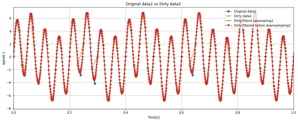
ダウンサンプリングをする際は、ダウンサンプリング前にエイリアシングフィルタを適用します。
# アップサンプリングしたデータをダウンサンプリングする処理
down_dirty_df = pd.DataFrame()
trans_nums = int((filtered_dirty_df['Time'].max() / (1 / f_temp)) * (f_trans / f_temp)) + 1
print('ダウンサンプリング後のデータ点数: '+ str(trans_nums))
down_dirty_df['Time'] = np.linspace(0, max(filtered_dirty_df['Time']), trans_nums)

for label in filtered_dirty_df:
    if label != 'Time':
        function = interpolate.interp1d(filtered_dirty_df['Time'], filtered_dirty_df[label], fill_value = 'extrapolate', kind = 'cubic')
        down_dirty_df[label] = function(down_dirty_df['Time'])
ダウンサンプリング後のデータ点数: 5000
# ダウンサンプリング後の時系列データのサンプリング間隔確認
print(down_dirty_df.head())
print(down_dirty_df.tail())
print(down_dirty_df.shape)
   Time     data1     data2
0  0.00  0.006593  0.081174
1  0.01  1.490991  5.329672
2  0.02  2.903705  4.210376
3  0.03  4.158394 -0.856879
4  0.04  5.180118 -2.724789
       Time     data1     data2
4995  49.95 -5.955735 -2.061151
4996  49.96 -5.136139  2.943741
4997  49.97 -4.200603  1.089745
4998  49.98 -2.917756 -3.740600
4999  49.99 -1.323847 -6.009585
(5000, 3)
fig, ax = plt.subplots(figsize = (16, 6))
ax.set_xlabel('Time[s]')
ax.set_ylabel('signal[-]')
ax.set_title('Original data1 vs Dirty data1')
ax.plot(df['Time'], df['data1'], label = 'Original data1', marker = 'D')
ax.plot(dirty_df['Time'], dirty_df['data1'], label = 'Dirty data1', marker='*')
ax.plot(filtered_up_dirty_df['Time'], filtered_up_dirty_df['data1'], label = 'Dirty filterd upsampling1', marker='+')
ax.plot(filtered_dirty_df['Time'], filtered_dirty_df['data1'], label = 'Dirty filtered before downsampling1', marker='v')
ax.plot(down_dirty_df['Time'], down_dirty_df['data1'], label = 'Dirty downsampling1', marker='<')
ax.legend(loc = 'upper right')
ax.set_xlim(0, 100 * (1 / samplerate))
ax.grid()
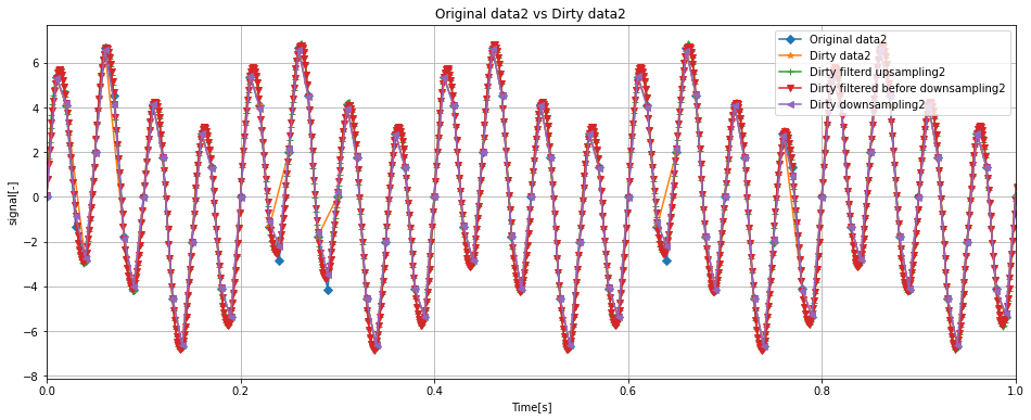
fig, ax = plt.subplots(figsize = (16, 6))
ax.set_xlabel('Time[s]')
ax.set_ylabel('signal[-]')
ax.set_title('Original data2 vs Dirty data2')
ax.plot(df['Time'], df['data2'], label = 'Original data2', marker = 'D')
ax.plot(dirty_df['Time'], dirty_df['data2'], label = 'Dirty data2', marker='*')
ax.plot(filtered_up_dirty_df['Time'], filtered_up_dirty_df['data2'], label = 'Dirty filterd upsampling2', marker='+')
ax.plot(filtered_dirty_df['Time'], filtered_dirty_df['data2'], label = 'Dirty filtered before downsampling2', marker='v')
ax.plot(down_dirty_df['Time'], down_dirty_df['data2'], label = 'Dirty downsampling2', marker='<')
ax.legend(loc = 'upper right')
ax.set_xlim(0, 100 * (1 / samplerate))
ax.grid()
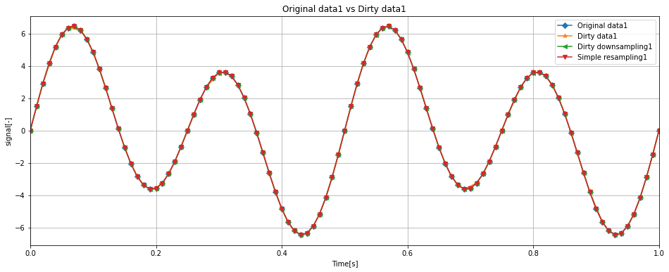
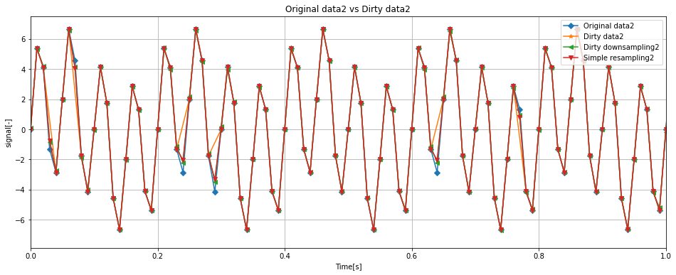
これで全ての処理が完了しました。
ここで、評価をしやすくするためにOriginal / Dirty / Dirty downsamplingに着目したグラフを表示します。
fig, ax = plt.subplots(figsize = (16, 6))
ax.set_xlabel('Time[s]')
ax.set_ylabel('signal[-]')
ax.set_title('Original data1 vs Dirty data1')
ax.plot(df['Time'], df['data1'], label = 'Original data1', marker = 'D')
ax.plot(dirty_df['Time'], dirty_df['data1'], label = 'Dirty data1', marker='*')
ax.plot(down_dirty_df['Time'], down_dirty_df['data1'], label = 'Dirty downsampling1', marker='<')
ax.legend(loc = 'upper right')
ax.set_xlim(0, 100 * (1 / samplerate))
ax.grid()

fig, ax = plt.subplots(figsize = (16, 6))
ax.set_xlabel('Time[s]')
ax.set_ylabel('signal[-]')
ax.set_title('Original data2 vs Dirty data2')
ax.plot(df['Time'], df['data2'], label = 'Original data2', marker = 'D')
ax.plot(dirty_df['Time'], dirty_df['data2'], label = 'Dirty data2', marker='*')
ax.plot(down_dirty_df['Time'], down_dirty_df['data2'], label = 'Dirty downsampling2', marker='<')
ax.legend(loc = 'upper right')
ax.set_xlim(0, 100 * (1 / samplerate))
ax.grid()
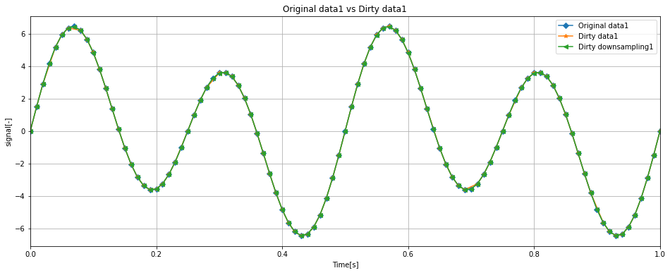
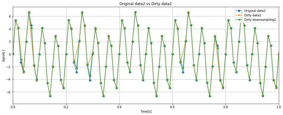
上記のグラフを見ると、data1についてはよく特徴をつかめていることがわかります。
一方で、data2についてはいくつかオリジナルに対して差分がある点が見られますが、Dirty downsamplingは良好に波形の特徴を掴んでいます。
信号に含まれる周波数に関してナイキスト周波数に近いものが多いとリサンプリングの精度が落ちるのかもしれないと考察しています。
# アップサンプリング後データの周波数解析
delta_f = 0.2# 周波数分解能(自分で決める)
Fs = int(f_temp / delta_f)
overlap_rate = 70  # オーバーラップ率
fft_array_up_dirty_data1, fft_axis_up_dirty_data1, fft_spectrum_up_dirty_data1, final_time_up_dirty_data1 = STFT_main(up_dirty_df['Time'].to_list(), up_dirty_df['data1'].to_list(), Fs, f_temp, overlap_rate, window_type="hanning", spectrum_type="AMP")
fft_array_up_dirty_data2, fft_axis_up_dirty_data2, fft_spectrum_up_dirty_data2, final_time_up_dirty_data2 = STFT_main(up_dirty_df['Time'].to_list(), up_dirty_df['data2'].to_list(), Fs, f_temp, overlap_rate, window_type="hanning", spectrum_type="AMP")
Execute FFT
Execute FFT
# ダウンサンプリング後データの周波数解析
delta_f = 0.2# 周波数分解能(自分で決める)
Fs = int(f_trans / delta_f)
overlap_rate = 70  # オーバーラップ率
fft_array_down_dirty_data1, fft_axis_down_dirty_data1, fft_spectrum_down_dirty_data1, final_time_down_dirty_data1 = STFT_main(down_dirty_df['Time'].to_list(), down_dirty_df['data1'].to_list(), Fs, f_trans, overlap_rate, window_type="hanning", spectrum_type="AMP")
fft_array_down_dirty_data2, fft_axis_down_dirty_data2, fft_spectrum_down_dirty_data2, final_time_down_dirty_data2 = STFT_main(down_dirty_df['Time'].to_list(), down_dirty_df['data2'].to_list(), Fs, f_trans, overlap_rate, window_type="hanning", spectrum_type="AMP")
Execute FFT
Execute FFT
fig, ax = plt.subplots(figsize = (16, 6))
ax.set_xlabel('f[Hz]')
ax.set_ylabel('Amplitude[v]')
ax.set_title('Comparison of Data1')
ax.plot(fft_axis_data1, fft_spectrum_data1, label = 'Original data1', marker = 'D')
ax.plot(fft_axis_dirty_data1, fft_spectrum_dirty_data1, label = 'Dirty data1', marker = '<')
ax.plot(fft_axis_up_dirty_data1, fft_spectrum_up_dirty_data1, label = 'dirty_up data1', marker = '*')
ax.plot(fft_axis_down_dirty_data1, fft_spectrum_down_dirty_data1, label = 'dirty_down data1', marker = 'v')


ax.legend(loc = 'upper right')
ax.set_xlim(0, 10)
ax.grid()


fig, ay = plt.subplots(figsize = (16, 6))
ay.set_xlabel('f[Hz]')
ay.set_ylabel('Amplitude[v]')
ay.set_title('Comparison of Data2')
ay.plot(fft_axis_data2, fft_spectrum_data2, label = 'Original data2', marker = 'D')
ay.plot(fft_axis_dirty_data2, fft_spectrum_dirty_data2, label = 'Dirty data2', marker = '<')
ay.plot(fft_axis_up_dirty_data2, fft_spectrum_up_dirty_data2, label = 'Dirty_up data2', marker = '*')
ay.plot(fft_axis_down_dirty_data2, fft_spectrum_down_dirty_data2, label = 'Dirty_down data2', marker = 'v')

ay.legend(loc = 'upper right')
ay.set_xlim(0, 30)
ay.grid()
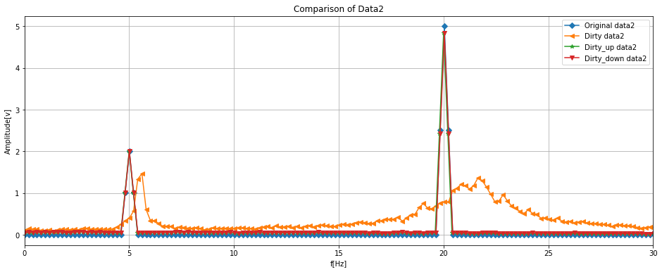
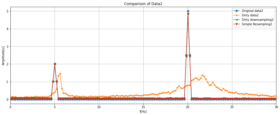
スペクトルを見てみると、Dirtyはかなり信号の質が悪化し、ピーク周波数がシフトしていたり裾野が広がっていました。
一方で、リサンプリングを行うことでこれが改善し、オリジナルに近いデータとなりました。
[9. まとめ]
一連の検討で下記のことが分かりました。
- interpolate関数を使うことで周波数の変換ができる
- 不等ピッチデータに対してもinterpolate関数は有効
- ただし、補間の設定は理論式をもとに理論的に実施したほうが良い
- 信号に含まれる周波数がナイキスト周波数に近いとリサンプリング精度が悪化する可能性
- もちろん、欠損しているデータが多ければ多いほどリサンプリングは困難になる
[10. おまけ: 周波数変換をする関数の紹介]
これまで周波数変換をする過程でローパスフィルタを随所で適用したり、周波数変換のための補間関数を作ってきました。
これらの処理を関数としたほうが便利になるため、1行で周波数変換を行う関数を実装しました。
本検討の最初に提示したローパスフィルタの関数と周波数変換をする関数を二つ使います。
[引数]
- df: 周波数変換したいデータフレームです。実際には、csvファイルなどを読み込んだデータになると思います。
- Timelabel: 入力したデータフレームにおける時系列のラベル名です。
- analysis_label: 周波数変換したいラベルをリストにして渡します。
- f_base: 入力したデータフレームのサンプリング周波数です。変換前の周波数とも言えます。
- f_trans: 変換後のサンプリング周波数です。
- mode: アップサンプリングかダウンサンプリングを指定します。(UP / DOWN)
- fill_value: 外挿オプションです。データの範囲外となる値を補完する場合、例えば0で埋めたり、一個前のサンプリング値で埋めることが出来ます。scipyに準拠しています。
- kind: 補間関数の設定です。scipyに準拠しています。
- fpass: ローパスフィルタの通過域端周波数です。
- fstop: 阻止域端周波数です
- gpass: 通過域最大損失量です
- gstop: 阻止域最大損失量です
[戻り値]
- リサンプリングされたデータフレームです
下記が実際の関数になります。
def butterlowpass(x, fpass, fstop, gpass, gstop, fs, dt, checkflag, labelname='Signal[-]'):
    from scipy import signal
    import matplotlib.pyplot as plt
    import numpy as np

    '''
    バターワースを用いたローパスフィルタ
    filtfilt関数により位相ずれを防ぐ
    (順方向と逆方向からフィルタをかけて位相遅れを相殺)
    :param x: 入力データ
    :param fpass: 通過域端周波数[Hz]
    :param fstop: 阻止域端周波数[Hz]
    :param gpass: 通過域最大損失量[dB]
    :param gstop: 阻止域最大損失量[dB]
    :param fs: サンプリング周波数[Hz]
    :param dt: サンプリング間隔[s]
    :param checkflag: グラフ生成ON/OFF
    :param labelname: 信号ラベル名
    :return: フィルター後データ
    '''

    print('Applying filter against: {0}...'.format(labelname))
    fn = 1 / (2 * dt)
    Wp = fpass / fn
    Ws = fstop / fn
    N, Wn = signal.buttord(Wp, Ws, gpass, gstop)
    b1, a1 = signal.butter(N, Wn, "low")
    y = signal.filtfilt(b1, a1, x)
    print(y)

    if checkflag == True:
        time = np.arange(x.__len__()) * dt
        plt.figure(figsize = (12, 5))
        plt.title('Comparison between signals')
        plt.plot(time, x, color='black', label='Raw signal')
        plt.plot(time, y, color='red', label='Filtered signal')
        plt.xlabel('Time[s]')
        plt.ylabel(labelname)
        plt.show()
    return y
def resample(df, Timelabel, analysis_label, f_base, f_trans, mode='UP', fill_value='extrapolate', kind='linear', fpass=None, fstop=None, gpass=None, gstop=None):
    from scipy import interpolate
    import pandas as pd
    filt_df, resampled_df = pd.DataFrame(),pd.DataFrame()
    trans_nums = int((df[Timelabel].max() / (1 / f_base)) * (f_trans / f_base)) + 1
    print('Base Sampling rate is {0} Hz. Transformed sampling rate is {1} Hz.'.format(f_base, f_trans))
    print('Max Time is {0} s'.format(df[Timelabel].max()))
    print('Number of sampling point is {0}. It will be {1} after resampling'.format(int(df[Timelabel].max() / (1 / f_base)),trans_nums))

    if mode == 'UP':
        if fpass == None:
            fpass = int(f_base / 2.56)
        if fstop == None:
            fstop = int(f_base / 2)
        if gpass == None:
            gpass = 3
        if gstop == None:
            gstop = 15
        resampled_df[Timelabel] = np.linspace(0, df[Timelabel].max(), trans_nums)
        for label in analysis_label:
            print('Resampling {0}...'.format(label))
            function = interpolate.interp1d(df[Timelabel], df[label], fill_value=fill_value, kind=kind)
            resampled_df[label] = function(resampled_df[Timelabel])

        filt_df[Timelabel] = resampled_df[Timelabel]
        for idx, labelname in enumerate(analysis_label):
            filt_df[labelname] = butterlowpass(x=resampled_df[labelname], fpass=fpass,
                                                                fstop=fstop,
                                                                gpass=gpass,
                                                                gstop=gstop,
                                                                fs=samplerate,
                                                                dt=1 / f_base,
                                                                checkflag=False,
                                                                labelname=labelname)
        return filt_df

    if mode == 'DOWN':
        if fpass == None:
            fpass = int(f_trans / 2.56)
        if fstop == None:
            fstop = int(f_trans / 2)
        if gpass == None:
            gpass = 3
        if gstop == None:
            gstop = 15

        filt_df[Timelabel] = df[Timelabel]
        for idx, labelname in enumerate(analysis_label):
            filt_df[labelname] = butterlowpass(x=resampled_df[labelname], fpass=fpass,
                                                                fstop=fstop,
                                                                gpass=gpass,
                                                                gstop=gstop,
                                                                fs=samplerate,
                                                                dt=1 / f_base,
                                                                checkflag=False,
                                                                labelname=labelname)
        resampled_df[Timelabel] = np.linspace(0, filt_df[Timelabel].max(), trans_nums)
        for label in analysis_label:
            print('Resampling {0}...'.format(label))
            function = interpolate.interp1d(filt_df[Timelabel], filt_df[label], fill_value=fill_value, kind=kind)
            resampled_df[label] = function(resampled_df[Timelabel])

        return resampled_df
    else:
        print('Please input correct mode')
        return None
[使い方]
- 時系列、data1、data2という名前の信号が格納されたdataframeがあると仮定
- サンプリング周波数は100Hzで計測時間は0 ~ 49.999秒。1000Hzに周波数変換する
- 解析したい信号はdata1、data2。つまりanalysis_label = ['data1', 'data2']
- Timelabelは'Time'
- f_base = 100, f_trans = 1000, f_pass = f_base / 2.56, f_stop = f_base / 2, gpass = 3, gstop = 15, mode = 'UP'
- fill_val = 'extrapolate', kind='linear'とする
注意点としては、ダウンサンプリング及びアップサンプリングする際のfpassとfstopの設定です。
ダウンサンプリングするときは変換後周波数のナイキスト周波数を、アップサンプリングするときは変換前周波数のナイキスト周波数を設定してください。
# データフレームを定義
# サンプリング周波数を100Hzとする
import numpy as np
import pandas as pd
samplerate = 100
f_trans = 1000
f1 = 2
f2 = 4
t = np.arange(0, 50, 1 / samplerate)
data1 = 2 * np.sin(2 * np.pi * f1 * t) + 5 * np.sin(2 * np.pi * f2 * t)


f3 = 5
f4 = 20
data2 = 2 * np.sin(2 * np.pi * f3 * t) + 5 * np.sin(2 * np.pi * f4 * t)

# DataFrame化
df = {}
df['Time'] = t
df['data1'] = data1
df['data2'] = data2
df = pd.DataFrame(df)
print(df.head())
print(df.tail())
   Time     data1     data2
0  0.00  0.000000  0.000000
1  0.01  1.494116  5.373317
2  0.02  2.906148  4.114497
3  0.03  4.158985 -1.320892
4  0.04  5.185147 -2.853170
       Time     data1     data2
4995  49.95 -5.930853 -2.000000
4996  49.96 -5.185147  2.853170
4997  49.97 -4.158985  1.320892
4998  49.98 -2.906148 -4.114497
4999  49.99 -1.494116 -5.373317
analysis_label = ['data1', 'data2']
resampled_df = resample(df, 'Time', analysis_label, samplerate, f_trans, mode='UP', fill_value='extrapolate', kind='linear', fpass=int(samplerate/2.56), fstop=int(samplerate/2), gpass=3, gstop=15)
Base Sampling rate is 100 Hz. Transformed sampling rate is 1000 Hz.
Max Time is 49.99 s
Number of sampling point is 4999. It will be 49991 after resampling
Resampling data1...
Resampling data2...
Applying filter against: data1...
[ 1.46982237e-04  1.49342951e-01  2.98854142e-01 ... -1.77658078e+00
 -1.63518943e+00 -1.49439370e+00]
Applying filter against: data2...
[ 4.97694903e-04  5.37150344e-01  1.07463566e+00 ... -5.12140586e+00
 -5.24759484e+00 -5.37304787e+00]
import matplotlib.pyplot as plt
fig, ax = plt.subplots(figsize = (16, 6))
ax.set_xlabel('Time[s]')
ax.set_ylabel('signal[-]')
ax.set_title('Original data1 vs Resampled data1')
ax.plot(df['Time'], df['data1'], label = 'Original data1', marker = 'D')
ax.plot(resampled_df['Time'], resampled_df['data1'], label = 'Resampled data1', marker='<')
ax.legend(loc = 'upper right')
ax.set_xlim(0, 100 * (1 / f_trans))
ax.grid()
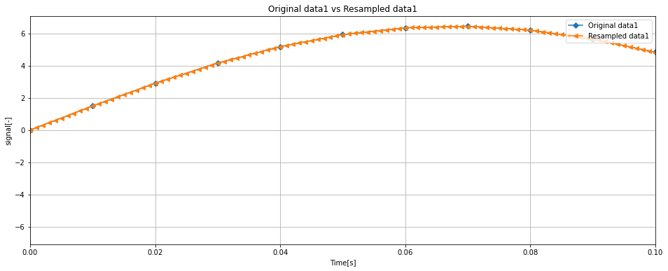
Original Dataに対して、Resampled dataはしっかりと細かいピッチでリサンプリングできています。
ここまで読んでいただきありがとうございました。本検討はこれで終了いたします。
(完全なJupyterコードはこちらです。https://github.com/cayk326/resample/blob/master/study_resample_method.ipynb)
[11. 追加検証]
本検討の7章以降で使用したデータは例えば下記のようなデータである。
Time, data1, data2
0, 1, 2
0.01, 1, 2
0.03, 3, 1
0.04, 3, 3
0.05, 2, 1
0.08, 6, 3
@carnage様から、このデータの場合はアップサンプリング->ダウンサンプリングを実施せずに
シンプルに狙いのサンプリングレートで補間できるのではという助言を頂いた。(ありがとうございます!)
これに関しての簡単な追加検証を以下で行った。
# 今一度dirty_dfを表示
print(dirty_df.head(10))
print(dirty_df.tail(10))
fig, ax = plt.subplots(figsize = (16, 6))
ax.set_xlabel('Time[s]')
ax.set_ylabel('signal[-]')
ax.set_title('Original data1 vs Dirty data1')
ax.plot(df['Time'], df['data1'], label = 'Original data1', marker = 'D')
ax.plot(dirty_df['Time'], dirty_df['data1'], label = 'Dirty data1', marker='*')
ax.legend(loc = 'upper right')
ax.set_xlim(0, 100 * (1 / samplerate))
ax.grid()

fig, ax = plt.subplots(figsize = (16, 6))
ax.set_xlabel('Time[s]')
ax.set_ylabel('signal[-]')
ax.set_title('Original data2 vs Dirty data2')
ax.plot(df['Time'], df['data2'], label = 'Original data2', marker = 'D')
ax.plot(dirty_df['Time'], dirty_df['data2'], label = 'Dirty data2', marker='*')
ax.legend(loc = 'upper right')
ax.set_xlim(0, 100 * (1 / samplerate))
ax.grid()
    Time     data1         data2
0   0.00  0.000000  0.000000e+00
1   0.01  1.494116  5.373317e+00
2   0.02  2.906148  4.114497e+00
4   0.04  5.185147 -2.853170e+00
5   0.05  5.930853  2.000000e+00
6   0.06  6.359228  6.657396e+00
8   0.08  6.212791 -1.763356e+00
9   0.09  5.662220 -4.137249e+00
10  0.10  4.841039 -2.204364e-15
11  0.11  3.805197  4.137249e+00
       Time     data1         data2
4989  49.89 -3.805197 -4.137249e+00
4990  49.90 -4.841039 -6.523358e-13
4991  49.91 -5.662220  4.137249e+00
4992  49.92 -6.212791  1.763356e+00
4994  49.94 -6.359228 -6.657396e+00
4995  49.95 -5.930853 -2.000000e+00
4996  49.96 -5.185147  2.853170e+00
4997  49.97 -4.158985  1.320892e+00
4998  49.98 -2.906148 -4.114497e+00
4999  49.99 -1.494116 -5.373317e+00

例えば、下記のような形で補間する。
Time, data1, data2
0, 1, 2
0.01, 1, 2
0.02, *, *
0.03, 3, 1
0.04, *, *
0.05, 2, 1
0.06, *, *
0.07, *, *
0.08, 6, 3
*を0で埋めてから補間する。
# リサンプリング
resample_dirty_df = pd.DataFrame()
trans_nums = int((dirty_df['Time'].max() / (1 / samplerate))) + 1
print('リサンプリング後のデータ点数: '+ str(trans_nums))
resample_dirty_df['Time'] = np.linspace(0, max(dirty_df['Time']), trans_nums)# truns_nums個分のデータ点数を使用して等差級数を作成
resample_dirty_df.head(10)

# 各データラベル(ここではdata1とdata2)に対して補間関数を作成し、データをリサンプリング
for label in dirty_df:
    if label != 'Time':
        function = interpolate.interp1d(dirty_df['Time'], dirty_df[label], fill_value = 0, kind = 'cubic')# 補間関数の作成
        resample_dirty_df[label] = function(resample_dirty_df['Time'])# リサンプリング
リサンプリング後のデータ点数: 5000
fig, ax = plt.subplots(figsize = (16, 6))
ax.set_xlabel('Time[s]')
ax.set_ylabel('signal[-]')
ax.set_title('Original data1 vs Dirty data1')
ax.plot(df['Time'], df['data1'], label = 'Original data1', marker = 'D')
ax.plot(dirty_df['Time'], dirty_df['data1'], label = 'Dirty data1', marker='*')
ax.plot(down_dirty_df['Time'], down_dirty_df['data1'], label = 'Dirty downsampling1', marker='<')
ax.plot(resmple_dirty_df['Time'], resample_dirty_df['data1'], label = 'Simple resampling', marker='v')
ax.legend(loc = 'upper right')
ax.set_xlim(0, 100 * (1 / samplerate))
ax.grid()

fig, ay = plt.subplots(figsize = (16, 6))
ay.set_xlabel('Time[s]')
ay.set_ylabel('signal[-]')
ay.set_title('Original data2 vs Dirty data2')
ay.plot(df['Time'], df['data2'], label = 'Original data2', marker = 'D')
ay.plot(dirty_df['Time'], dirty_df['data2'], label = 'Dirty data2', marker='*')
ay.plot(down_dirty_df['Time'], down_dirty_df['data2'], label = 'Dirty downsampling2', marker='<')
ay.plot(resmple_dirty_df['Time'], resample_dirty_df['data2'], label = 'Simple resampling', marker='v')
ay.legend(loc = 'upper right')
ay.set_xlim(0, 100 * (1 / samplerate))
ay.grid()
緑線がdirty_dfに対して、一度アップサンプリングを実施しダウンサンプリングしたものであり、
赤線がdirty_dfに対して、狙いのサンプリングレートで時間列を構成し直し、シンプルに補間を行ったものである。
時系列波形を見ると、赤と緑線に大きな違いは見られずにほぼ一致する形となった。
これならばアップサンプリング->ダウンサンプリングせずに、シンプルにリサンプリングしたほうが良さそうだ。
# リサンプリング後データの周波数解析
delta_f = 0.2# 周波数分解能(自分で決める)
Fs = int(samplerate / delta_f)
overlap_rate = 70  # オーバーラップ率
fft_array_resample_dirty_data1, fft_axis_resample_dirty_data1, fft_spectrum_resample_dirty_data1, final_time_resample_dirty_data1 = STFT_main(resample_dirty_df['Time'].to_list(), resample_dirty_df['data1'].to_list(), Fs, samplerate, overlap_rate, window_type="hanning", spectrum_type="AMP")
fft_array_resample_dirty_data2, fft_axis_resample_dirty_data2, fft_spectrum_resample_dirty_data2, final_time_resample_dirty_data2 = STFT_main(resample_dirty_df['Time'].to_list(), resample_dirty_df['data2'].to_list(), Fs, samplerate, overlap_rate, window_type="hanning", spectrum_type="AMP")
Execute FFT
Execute FFT
fig, ax = plt.subplots(figsize = (16, 6))
ax.set_xlabel('f[Hz]')
ax.set_ylabel('Amplitude[v]')
ax.set_title('Comparison of Data1')
ax.plot(fft_axis_data1, fft_spectrum_data1, label = 'Original data1', marker = 'D')
ax.plot(fft_axis_dirty_data1, fft_spectrum_dirty_data1, label = 'Dirty data1', marker = '*')
ax.plot(fft_axis_down_dirty_data1, fft_spectrum_down_dirty_data1, label = 'Dirty downSampling1', marker = '<')
ax.plot(fft_axis_resample_dirty_data1, fft_spectrum_resample_dirty_data1, label = 'Simple Resampling1', marker = 'v')


ax.legend(loc = 'upper right')
ax.set_xlim(0, 10)
ax.grid()


fig, ay = plt.subplots(figsize = (16, 6))
ay.set_xlabel('f[Hz]')
ay.set_ylabel('Amplitude[v]')
ay.set_title('Comparison of Data2')
ay.plot(fft_axis_data2, fft_spectrum_data2, label = 'Original data2', marker = 'D')
ay.plot(fft_axis_dirty_data2, fft_spectrum_dirty_data2, label = 'Dirty data2', marker = '*')
ay.plot(fft_axis_down_dirty_data2, fft_spectrum_down_dirty_data2, label = 'Dirty downsampling2', marker = '<')
ay.plot(fft_axis_resample_dirty_data2, fft_spectrum_resample_dirty_data2, label = 'Simple Resampling2', marker = 'v')


ay.legend(loc = 'upper right')
ay.set_xlim(0, 30)
ay.grid()

更に、FFT結果も緑線と赤線はほぼ重なる結果となった。