深層学習day3

深層学習

確認テスト

サイズ5×5の入力画像を、サイズ3×3のフィルタで畳み込んだ時の出力画像のサイズを答えよ。スライドは2、パディングは1とする。
回答
3*3

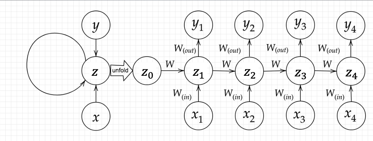
Section1：再帰型ニューラルネットワークの概念

• 時系列データなど、前の結果が次の結果に影響するようなデータに対応可能なニューラルネットワーク。
• 自然言語処理の、テキスト処理の分野（翻訳やチャットボット、要約など）において重要な技術だった。（現在はTransformerなど、再起的な構造を持たないものが主流になっている。）

確認テスト

RNNのネットワークには大きくわけて3つの重みがある。1つは入力から現在の中間層を定義する際にかけられる重み、1つは中間層から出力を定義する際にかけられる重みである。残り1つの重みについて説明せよ。
回答
前の時刻の出力にかけられる重み

確認テスト

連鎖律の原理を使い、dz/dxを求めよ。

z = t^2\\
t = x+y

回答

\frac{dz}{dx}=\frac{dz}{dt}\frac{dt}{dx}=2t*1=2(x+y)

確認テスト

下図のy1をx・s0・s1・win・w・woutを用いて数式で表せ。※バイアスは任意の文字で定義せよ。※また中間層の出力にシグモイド関数g(x)を作用させよ。

回答

z_1 = sigmoid(s_0W+x_1W_{in}+b)\\
y_1=sigmoid(z_1W_{out}+c)

実装演習

import numpy as np
from common import functions
import matplotlib.pyplot as plt


def d_tanh(x):
    return 1/(np.cosh(x) ** 2)

# データを用意
# 2進数の桁数
binary_dim = 8
# 最大値 + 1
largest_number = pow(2, binary_dim)
# largest_numberまで2進数を用意
binary = np.unpackbits(np.array([range(largest_number)],dtype=np.uint8).T,axis=1)

input_layer_size = 2
hidden_layer_size = 16
output_layer_size = 1

weight_init_std = 1
learning_rate = 0.1

iters_num = 10000
plot_interval = 100

# ウェイト初期化 (バイアスは簡単のため省略)
W_in = weight_init_std * np.random.randn(input_layer_size, hidden_layer_size)
W_out = weight_init_std * np.random.randn(hidden_layer_size, output_layer_size)
W = weight_init_std * np.random.randn(hidden_layer_size, hidden_layer_size)
# Xavier
# W_in = np.random.randn(input_layer_size, hidden_layer_size) / (np.sqrt(input_layer_size))
# W_out = np.random.randn(hidden_layer_size, output_layer_size) / (np.sqrt(hidden_layer_size))
# W = np.random.randn(hidden_layer_size, hidden_layer_size) / (np.sqrt(hidden_layer_size))
# He
# W_in = np.random.randn(input_layer_size, hidden_layer_size) / (np.sqrt(input_layer_size)) * np.sqrt(2)
# W_out = np.random.randn(hidden_layer_size, output_layer_size) / (np.sqrt(hidden_layer_size)) * np.sqrt(2)
# W = np.random.randn(hidden_layer_size, hidden_layer_size) / (np.sqrt(hidden_layer_size)) * np.sqrt(2)


# 勾配
W_in_grad = np.zeros_like(W_in)
W_out_grad = np.zeros_like(W_out)
W_grad = np.zeros_like(W)

u = np.zeros((hidden_layer_size, binary_dim + 1))
z = np.zeros((hidden_layer_size, binary_dim + 1))
y = np.zeros((output_layer_size, binary_dim))

delta_out = np.zeros((output_layer_size, binary_dim))
delta = np.zeros((hidden_layer_size, binary_dim + 1))

all_losses = []

for i in range(iters_num):
    
    # A, B初期化 (a + b = d)
    a_int = np.random.randint(largest_number/2)
    a_bin = binary[a_int] # binary encoding
    b_int = np.random.randint(largest_number/2)
    b_bin = binary[b_int] # binary encoding
    
    # 正解データ
    d_int = a_int + b_int
    d_bin = binary[d_int]
    
    # 出力バイナリ
    out_bin = np.zeros_like(d_bin)
    
    # 時系列全体の誤差
    all_loss = 0    
    
    # 時系列ループ
    for t in range(binary_dim):
        # 入力値
        X = np.array([a_bin[ - t - 1], b_bin[ - t - 1]]).reshape(1, -1)
        # 時刻tにおける正解データ
        dd = np.array([d_bin[binary_dim - t - 1]])
        
        u[:,t+1] = np.dot(X, W_in) + np.dot(z[:,t].reshape(1, -1), W)
        z[:,t+1] = functions.sigmoid(u[:,t+1])
#         z[:,t+1] = functions.relu(u[:,t+1])
#         z[:,t+1] = np.tanh(u[:,t+1])    
        y[:,t] = functions.sigmoid(np.dot(z[:,t+1].reshape(1, -1), W_out))


        #誤差
        loss = functions.mean_squared_error(dd, y[:,t])
        
        delta_out[:,t] = functions.d_mean_squared_error(dd, y[:,t]) * functions.d_sigmoid(y[:,t])        
        
        all_loss += loss

        out_bin[binary_dim - t - 1] = np.round(y[:,t])
    
    
    for t in range(binary_dim)[::-1]:
        X = np.array([a_bin[-t-1],b_bin[-t-1]]).reshape(1, -1)        

        delta[:,t] = (np.dot(delta[:,t+1].T, W.T) + np.dot(delta_out[:,t].T, W_out.T)) * functions.d_sigmoid(u[:,t+1])
#         delta[:,t] = (np.dot(delta[:,t+1].T, W.T) + np.dot(delta_out[:,t].T, W_out.T)) * functions.d_relu(u[:,t+1])
#         delta[:,t] = (np.dot(delta[:,t+1].T, W.T) + np.dot(delta_out[:,t].T, W_out.T)) * d_tanh(u[:,t+1])    

        # 勾配更新
        W_out_grad += np.dot(z[:,t+1].reshape(-1,1), delta_out[:,t].reshape(-1,1))
        W_grad += np.dot(z[:,t].reshape(-1,1), delta[:,t].reshape(1,-1))
        W_in_grad += np.dot(X.T, delta[:,t].reshape(1,-1))
    
    # 勾配適用
    W_in -= learning_rate * W_in_grad
    W_out -= learning_rate * W_out_grad
    W -= learning_rate * W_grad
    
    W_in_grad *= 0
    W_out_grad *= 0
    W_grad *= 0
    

    if(i % plot_interval == 0):
        all_losses.append(all_loss)        
        print("iters:" + str(i))
        print("Loss:" + str(all_loss))
        print("Pred:" + str(out_bin))
        print("True:" + str(d_bin))
        out_int = 0
        for index,x in enumerate(reversed(out_bin)):
            out_int += x * pow(2, index)
        print(str(a_int) + " + " + str(b_int) + " = " + str(out_int))
        print("------------")

lists = range(0, iters_num, plot_interval)
plt.plot(lists, all_losses, label="loss")
plt.show()

結果

iters:0
Loss:2.327797937294226
Pred:[1 1 1 1 1 1 1 1]
True:[0 0 0 1 0 0 1 1]
7 + 12 = 255
------------
iters:100
Loss:0.9815474172490911
Pred:[0 0 0 0 0 1 0 1]
True:[0 0 1 0 1 1 0 0]
44 + 0 = 5
------------
iters:200
Loss:0.9048102021703512
Pred:[1 1 1 1 1 1 1 1]
True:[1 0 1 0 1 1 1 0]
88 + 86 = 255
------------
.
.
.
------------
iters:9700
Loss:0.0003353745712332112
Pred:[1 0 1 0 1 1 0 0]
True:[1 0 1 0 1 1 0 0]
121 + 51 = 172
------------
iters:9800
Loss:0.00039447498051377794
Pred:[1 1 0 0 0 0 0 0]
True:[1 1 0 0 0 0 0 0]
97 + 95 = 192
------------
iters:9900
Loss:0.002013425728620699
Pred:[0 1 1 1 1 0 1 0]
True:[0 1 1 1 1 0 1 0]
38 + 84 = 122
------------

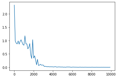
しっかりと学習できている。

Section2：LSTM

• RNNは時系列を遡れば遡るほど、勾配が消失していくため長い時系列の学習が困難。
• 入力ゲート、出力ゲート、忘却ゲートを用いて過去の情報を保持、忘却を行う。
• パラメータ数が多く計算負荷が高いが精度が高い。

確認テスト

シグモイド関数を微分した時、入力値が0の時に最大値をとる。その値として正しいものを選択肢から選べ。
（1）0.15（2）0.25（3）0.35（4）0.45
回答

(sigmoid(x))'=(1-sigmoid(x))sigmoid(x)\\
(1-sigmoid(0))sigmoid(0)=(1-0.5)0.5=0.25

確認テスト

以下の文章をLSTMに入力し空欄に当てはまる単語を予測したいとする。文中の「とても」という言葉は空欄の予測においてなくなっても影響を及ぼさないと考えられる。このような場合、どのゲートが作用すると考えられるか。
「映画おもしろかったね。ところで、とてもお腹が空いたから何か____。」
回答
忘却ゲート

Section3：GRU

• LSTMと同様にRNNの一種であり、単純なRNNにおいて問題となる勾配消失問題を解決し、長期的な依存関係を学習することができる。
• 従来のLSTMでは、パラメータが多数存在していたため、計算負荷が大きかった。
• GRUは、そのパラメータを大幅に削減し、精度は同等またはそれ以上が望める様になった構造。

確認テスト

LSTMとCECが抱える課題について、それぞれ簡潔に述べよ。
回答
LSTMはパラメータの数が多く計算コストも高い。
CECはパラメータ更新が行われない

確認テスト

LSTMとGRUの違いを簡潔に述べよ。
LSTMは入力ゲート、出力ゲート、忘却ゲートをもちパラメータの数が多い。
GRUはリセットゲートと更新ゲートを持ちパラメータの数が少ない。

Section4：双方向RNN

• 過去の情報だけでなく、未来の情報を加味することで、精度を向上させるためのモデル
• 文章推敲や機械翻訳等に用いられる。
• 順方向、逆方向の2つのRNNを組み合わせて使う。
• RNNの代わりにLSTMを用いることも多い。

Section5：Seq2Seq

• Encoder-Decoderモデルの一種を指す。
• 機械対話や、機械翻訳などに使用されている。
• Encoderの最終状態をDecoderの初期状態にすることで元の文を元に文を生成できるようにする。
• Decoderは生成した単語を元に次の単語を出力する。

確認テスト

下記の選択肢から、seq2seqについて説明しているものを選べ。
（1）時刻に関して順方向と逆方向のRNNを構成し、それら2つの中間層表現を特徴量として利用するものである。
（2）RNNを用いたEncoder-Decoderモデルの一種であり、機械翻訳などのモデルに使われる。
（3）構文木などの木構造に対して、隣接単語から表現ベクトル（フレーズ）を作るという演算を再帰的に行い（重みは共通）、文全体の表現ベクトルを得るニューラルネットワークである。
（4）RNNの一種であり、単純なRNNにおいて問題となる勾配消失問題をCECとゲートの概念を導入することで解決したものである。
回答
(2)

確認テスト

seq2seqとHRED、HREDとVHREDの違いを簡潔に述べよ。
回答
seq2seqは文脈を無視した応答になってしまうが、HREDは過去の会話を元に、文脈を考慮した応答になる。
HREDは同じコンテキストを与えると同じ答えを出してしまい多様性がなくなる。また短い答えを選ぶ傾向がある。
VHREDはVAEの概念を利用し、多様な出力を行える。

確認テスト

VAEに関する下記の説明文中の空欄に当てはまる言葉を答えよ。
自己符号化器の潜在変数に____を導入したもの。
回答
確率分布z∼N(0,1)

Section6：Word2vec

• RNNでは、単語のような可変長の文字列をNNに与えることはできないため、固定長のベクトルに変換する。
• 「単語の意味は周囲の単語によって形成される」という分布仮説に基づいて学習する。
• CBOWとSkip-gramの2つがある。

Section7：Attention Mechanism

• 「入力と出力のどの単語が関連しているのか」の関連度を学習する仕組み。
• 固定長のベクトルにEncoderの全ての情報に圧縮するのは無理があるためEncoderの全ての状態をDecoderが利用できるようにする。

確認テスト

RNNとword2vec、seq2seqとAttentionの違いを簡潔に述べよ。
回答
RNNはシーケンスデータをベクトルに変換するニューラルネットワークでword2vecは単語をベクトルに変換するニューラルネットワーク。
seq2seqはEncoderの最後の状態のみをDecoderに渡すが、Attentionは全ての状態をDecoderに渡す。